Aims

In this tutorial I will show you how you can use PLUMED and metadynamics to study the binding between a ion and a dinucleotide.

Objectives

Once this tutorial is completed students will

Know how to enhance binding between molecules using metadynamics.
Know how to analyze metadynamics simulations.
Know how to compute standard affinities.

Resources

The reference trajectory and other files can be obtained at this path

wget https://github.com/plumed/lugano2019/raw/master/lugano-6b.tgz

This tutorial has been tested on v2.5 but it should also work with other versions of PLUMED.

Introduction

For this tutorial we will consider a practical application. The system is actually taken from [37]. It is one of the simplest systems studied in that paper, namely a guanine dinucleotide monophosphate binding a Mg ion. This is a very simple binding event, but a very similar procedure might be used to study binding of a ligand on a protein. The reason why this exercise is particularly simple is that instead of the ligand we have a single ion, thus with no internal degree of freedom, and instead of a protein with a complex binding pocket we have a dinucleotide. We are also assuming to know which is the proper binding site, since we can easily guess that the most stable binding will happen on the phosphate.

Since running these simulations on your laptop would take too long, you will start with the output files obtained with a decently long simulation and analyze them.

Warning: The trajectory is too short (approx 20ns) to obtain converged results! To get statistically significant numbers, please run it longer.

Before continuing, please read carefully the plumed.dat file that was used to produce the simulation, since there you will find all the explanations about which variables were biased and how.

In case you want to do analysis with python, you can use the included plumed_pandas.py module, which is a preview of a feature that will be available in plumed 2.6. It requires pandas to be installed (use conda install pandas) and allows to extract columns from a COLVAR file by name. It works in this way:

> import plumed_pandas
> import matplotlib.pyplot as plt
> df=plumed_pandas.read_as_pandas("COLVAR")
# shows the head of the file:
> df.head()
# plot distance between Mg and phosphate
> plt.plot(df["dp"][:],".")
# plot coordination number of Mg with water
> plt.plot(df["cn"][:],".")

Exercises

Exercise 1: Computing the free energy as a function of the biased variables.

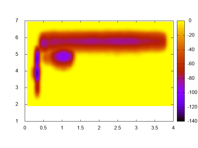
As the title says, just compute the free-energy landscape as a function of the biased collective variable (namely, distance between the Mg ion and the phosphate and coordination number of the Mg ion with water oxygen atoms). You should just use sum_hills with the usual options. In order to visualize the result with gnuplot you might use something like this:

gnuplot> set pm3d map
gnuplot> sp "fes.dat" u 1:2:3

You should obtain a plot similar to this one:

Free energy as a function of distance from phosphate and coordination with water

Exercise 2: Visualizing the trajectory

This exercise is optional and is not needed to continue with the next points. However, it is a very good idea to do it in order to have a better understanding of what the system is doing!

Beware that the periodic boundary conditions were broken. You can adjust them using PLUMED with an input like this one (please fill the gaps)

MOLINFO STRUCTURE=conf.pdb
WHOLEMOLECULES ENTITY0=@nucleic
c: CENTER ATOMS=@nucleic
mg:  GROUP ATOMS=__FILL__ # find the serial number of the Mg ion
WRAPAROUND AROUND=c ATOMS=mg

# check documentation of WRAPAROUND!
# you should also know how many atoms make a water molecule
WRAPAROUND AROUND=c ATOMS=@water GROUPBY=__FILL__

# dump your trajectory
DUMPATOMS ATOMS=@mdatoms FILE=whole.xtc
# writing all atoms you will be able to reuse the same pdb for opening.
# e.g. vmd conf.pdb whole.xtc

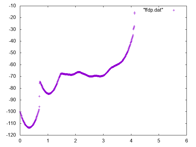
Exercise 3: Reweighting your free energy

Now reweight your free energy and compute it as a function of:

distance between Mg and phosphate
distance between Mg and geometric center of RNA
coordination number between Mg and water

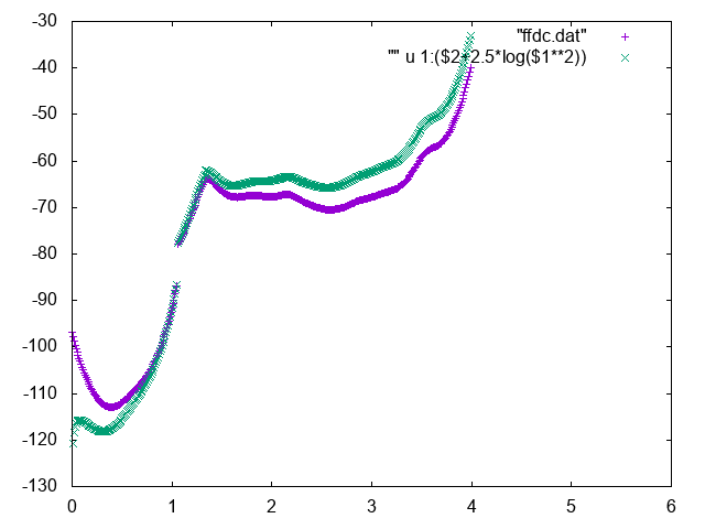
The free energy as a function of the distance between Mg and geometric center of RNA can be used to identify the bulk region. In order to do so, normalize it adding the correct entropic term \(k_BT\log d^2\), and find a region where the free energy is approximately constant to represent the bulk region. You can for instance use the following commands in gnuplot

gnuplot> p "fes_dc" u 1:2 , "" u 1:($2+2.5*log($1**2))

Below you can find reference results

Free energy as a function of distance between Mg and phosphate

Free energy as a function of distance between Mg and RNA center

Free energy as a function of coordination between Mg and water oxygens

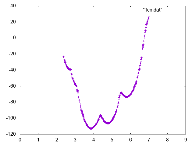
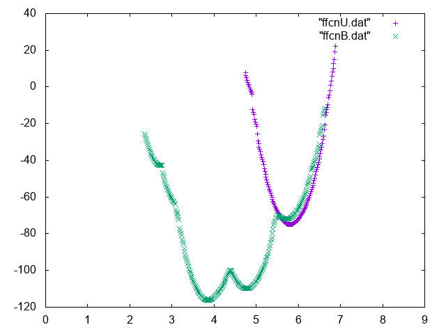
Also try to compute conditional free energies:

coordination number between Mg and water assuming Mg is bound to phosphate.
coordination number between Mg and water assuming Mg is in the bulk.

A possible way to do so you can use UPDATE_IF to extract portions of trajectory such that the Mg is bound or unbound.

Below you can find reference results

Free energy as a function of coordination between Mg and water oxygens, both for Mg bound and unbound

Exercise 4: Standard affinity

Now use the weights that you computed in the previous exercise to compute the absolute binding affinity of the Mg to the phosphate. In order to do so you should compute the relative probability of seeing the Mg bound to the phosphate and in the bulk region and normalize to 1 mol/M concentration.

For instance, if you define bulk the region between 1.5 and 2.5 nm, you should divide the weight of the unbound state by a factor \( \frac{4\pi}{3}(2.5^3-1.5^3)/V_{mol} \) where \(V_{mol}=1.66 nm^3\) is the volume corresponding to the inverse of 1 mol/L concentration. The absolute binding affinity is then defined as \(-k_BT \log \frac{w_B}{w_U} \). You should obtain a value of approximately 50.4 kj/mol

Warning: The trajectory is too short (approx 20ns) to obtain converged results! To get statistically significant numbers, please run it longer. Also notice that the result might depend a lot on the used force field.