 |
|
|
| |
|
|
The aim of this tutorial is to give you a quick introduction to the PLUMED syntax and to some of the types of calculations that can be done with PLUMED. It was prepared for a two and a half hour session on PLUMED in the following CECAM extended software development workshop on topics in classical MD:
https://www.cecam.org/workshop-1802.html
This tutorial is very straightforward and not at all exhaustive. In fact it skims over many of the subtleties associated with performing these types of calculations using PLUMED. We have thus suggested additional topics that you might like to look into throughout the tutorial in order to take this further.
If you are interested in using the techniques described in the tutorial in your own work a good starting point might be to read the chapter we wrote about using metadynamics from within PLUMED:
https://arxiv.org/abs/1812.08213
Once this tutorial is completed students will be able to:
The TARBALL for this project contains the following files:
This tutorial has been tested on v2.5 but it should also work with other versions of PLUMED.
Also notice that the .solutions direction of the tarball contains correct input files for the exercises. Please only look at these files once you have tried to solve the problems yourself. Similarly the tutorial below contains questions for you to answer that are shown in bold. You can reveal the answers to these questions by clicking on links within the tutorial but you should obviously try to answer things yourself before reading these answers.
In this tutorial we are going to study a very simple physical system; namely, seven Lennard Jones atoms in a two dimensional space. This simple system has been extensively studied as has often been used to benchmark new simulation techniques. In addition, the potential energy landscape has been fully characterized and it is known that only the four structurally-distinct minima shown below exist:
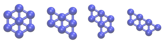
In the exercises that follow we are going to learn how to use PLUMED to determine the relative free energies of these four structures by running molecular dynamics simulations.
Before completing the following exercises you will need to download and install PLUMED. In addition, you will need to ensure that the PLUMED executable can be found within your path.
You can download PLUMED from:
http://www.plumed.org/get-it or https://github.com/plumed/plumed2
If you are running PLUMED on a Mac you can install the executable directly using macports and the command:
sudo port install plumed
If you download the source code you can find instructions on compilation in the PLUMED page on Installation. If you run make install PLUMED or install with macports PLUMED will be within your path.
If, however, you do not wish to do a make install you can simple make PLUMED. You can then add the location of the PLUMED executable to your path by issuing the command:
source sourceme.sh
from within the plumed2 directory.
PLUMED is primarily used as a plugin to other larger molecular dynamics codes. Mainly for software testing and educational purposes, however, we do have an MD code with a rather limited set of options within PLUMED. You can run this code by issuing the command:
plumed simplemd < in
where in here is the input file from the tar ball for this tutorial, which is shown below:
nputfile input.xyz
outputfile output.xyz
temperature 0.5
tstep 0.005
friction 0.1
forcecutoff 2.5
listcutoff  3.0
ndim 2
nstep 200000
nconfig 1000 trajectory.xyz
nstat   1000 energies.dat
This input instructs PLUMED to perform 200000 steps of MD at a temperature of \(k_B T = 0.5 \epsilon\) starting from the configuration in input.xyz. The timestep in this simulation is 0.005 \(\sqrt{\epsilon}{m\sigma^2}\) and the temperature is kept fixed using a Langevin thermostat with a relaxation time of \(0.1 \sqrt{\epsilon}{m\sigma^2}\). Trajectory frames are output every 1000 MD steps to a file called trajectory.xyz. Notice also that in order to run the calculation above you need to provide an empty file called plumed.dat. This file is the input file to the PLUMED plugin itself, which, because this file is empty, is doing nothing when we run the calculation above.
Run a calculation using simplemd and the input above and visualize the trajectory that is output. Describe what happens during this calculation and explain why this is happening.
You should observe that all the atoms fly apart early on in the simulation and that the cluster evaporates. The cluster evaporates because at a temperature of \(k_B T = 0.5 \epsilon\) the gas state has a lower free energy than than the cluster state. To learn more: What happens
You can visualize what occurs during the trajectory by using a visualization package such as VMD (https://www.ks.uiuc.edu/Research/vmd/). If you are using VMD you can see the MD trajectory by using the command:
vmd trajectory.xyz
Change the parameters in the input file for simplemd so as to prevent the cluster from evaporating.
To learn more: No evaporation
To prevent the cluster from evaporating you need to lower the temperature in the file in. The cluster will not evaporate if the temperature is set equal to \(k_B T = 0.2 \epsilon\).
If we lower the temperature of the simulation very little will happen. Yes the cluster will no longer evaporate but at the same time we will not see any transitions between the various basins in this energy landscape. In this section we are thus going to see how we can use PLUMED to add a bias potential that can prevent the cluster from exploring gaseous configurations that do not interest us. In other words, we are going to see how we can use PLUMED to add restraints that will prevent the cluster from evaporating. Before getting on to that, however, we first need to understand a little about how the PLUMED input file works. As explained in The structure of a PLUMED input file and Getting Started when you write a PLUMED input file you are writing a script that calculates functions of the atomic positions.
Read the description of the PLUMED input syntax in the linked pages in the paragraph above and then attempt the exercise that follows
We are going to prevent the cluster from evaporating by adding a restraint on all the atoms so as to prevent them from moving more than \(2\sigma\) from the center of mass of the cluster. As the masses of all the atoms in the cluster are the same we can compute the position of the center of mass using:
\[ \mathbf{x}_\textrm{com} = \frac{1}{N} \sum_{i=1}^N \mathbf{x}_i \]
where \(\mathbf{x}_i\) is the position of the \(i\)th atom. The distance between the \(i\)th atom and the position of this center of mass, \(d_i\), can be computed using Pythagoras' theorem. These distances are then restrained by using the following potential:
\[ V(d_i) = \begin{cases} 100*(d_i-2.0)^2 & \textrm{if} \quad d_i > 2 \\ 0 & \textrm{otherwise} \end{cases} \]
as you can see this potential has no effect on the dynamics when these distances are less than 2 \(\epsilon\). If any atom is more than 2 \(\epsilon\) from the center of mass, however, this potential will drive it back towards the center of mass. The following cell contains a skeleton input file for PLUMED that gets it to calculate and apply this bias potential.
# this optional command tells VIM that this is a PLUMED file and to color the text accordingly
# vim: ft=plumed

# This tells PLUMED we are using Lennard Jones units
UNITS NATURAL

# Calculate the position of the center of mass.  We can then refer to this position later in the input using the label com.
com: COM __FILL__

# Add the restraint on the distance between com and the first atom
d1: DISTANCE __FILL__
UPPER_WALLS ARG=d1 __FILL__

# Add the restraint on the distance between com and the first atom
d2: DISTANCE __FILL__
UPPER_WALLS  __FILL__

# Add the restraint on the distance between com and the first atom
d3: DISTANCE __FILL__
UPPER_WALLS __FILL__

# Add the restraint on the distance between com and the first atom
d4: DISTANCE __FILL__
UPPER_WALLS __FILL__

# Add the restraint on the distance between com and the first atom
d5: DISTANCE __FILL__
UPPER_WALLS __FILL__

# Add the restraint on the distance between com and the first atom
d6: DISTANCE __FILL__
UPPER_WALLS __FILL__

# Add the restraint on the distance between com and the first atom
d7: DISTANCE __FILL__
UPPER_WALLS __FILL__
Copy and paste the content above into the file plumed.dat and then fill in the blanks by looking up the documentation for these actions online and by reading the description of the calculation that you are to run above. Once you have got a working plumed.dat file run a calculation using simplemd again at a temperature of \(k_B T = 0.2 \epsilon\) and check to see if the bias potential is indeed preventing the cluster from evaporating.
Try the following exercises if you have time and if you wish to take this exercise further:
We can easily determine if there are transitions between the four possible minima in the Lennard-Jones-seven potential energy landscape by monitoring the second and third central moments of the distribution of coordination numbers. The \(n\)th central moment of a set of numbers, \(\{X_i\}\) can be calculated using:
\[ \mu^n = \frac{1}{N} \sum_{i=1}^N ( X_i - \langle X \rangle )^n \qquad \textrm{where} \qquad \langle X \rangle = \frac{1}{N} \sum_{i=1}^N X_i \]
Furthermore, we can compute the coordination number of our Lennard Jones atoms using:
\[ c_i = \sum_{i \ne j } \frac{1 - \left(\frac{r_{ij}}{1.5}\right)^8}{1 - \left(\frac{r_{ij}}{1.5}\right)^{16} } \]
where \(r_{ij}\)__FILL__ is the distance between atom \(i\) and atom \(j\). The following cell contains a skeleton input file for PLUMED that gets it to calculate and print the values these two quantities take every 100 time steps to a file called colvar.
c1: COORDINATIONNUMBER SPECIES=__FILL__ MOMENTS=__FILL__ SWITCH={RATIONAL __FILL__ }
PRINT ARG=__FILL__ FILE=colvar STRIDE=100
Copy and paste the content above into your plumed.dat file after the lines that you added in the previous exercise that added the restraints to stop the cluster from evaporating. Fill in the blanks in the input above and, once you have a working plumed.dat file, run a calculation using simplemd at a temperature of \(k_B T = 0.2 \epsilon\). Once you have generated the trajectory plot the time series of second and third moment values using gnuplot or some other plotting package.
To learn more: Example time series
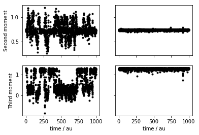 Time series for the second and third moments of the distribution of coordination numbers for two trajectories of Lennard Jones 7. The time series on the left was computed from a trajectory that was performed at a temperature of 0.2, while the two time series on the right were computed at a temperature of 0.1. You can see that at the higher temperature there are jumps between distinct minima in the energy landscape. At the lower temperature, however, the system remains trapped in a single basin in the energy lanscape
Try the following exercises if you have time and if you wish to take this exercise further:
When you plotted the time series for the collective variables in the previous exercise you should have seen that the values of these collective variables fluctuate around a number of different constant values for long periods of time. There are then infrequent jumps and after these jumps the value of the collective variable settles down and begins to fluctuate around a different constant value. There are jumps in the value of the CV whenever the system moves from one minimums illustrated above to another. What we would ideally like to extract from our simulation are the relative free energies of these various minimums. From elementary statistical mechanics, however, we know that the free energy is given by:
\[ F(s) = -k_B T \ln P(s) \]
Consequently, if we can extract an estimate of the probability that the CVs take particular values, \(s\), then we can get an estimate of the free energy. Extracting an estimate that for the probability that the collective variables take a particular value is easy, however. We just need to construct a histogram from the CV values that the system took during the trajectory. The following cell contains a skeleton input file for PLUMED that gets it to estimate this histogram and that converts and outputs this estimate of the histogram to a file called fes.dat.
hh: HISTOGRAM __FILL__ __FILL__=-1.0,-1.0 __FILL__=1.5,1.5 GRID_BIN=300,300 __FILL__=DISCRETE STRIDE=100
fes: CONVERT_TO_FES GRID=_FILL__ __FILL__=0.2
DUMPGRID GRID=__FILL__ FILE=fes.dat
Copy and paste the content above into your plumed.dat file after the lines that you added in the previous two exercises. Fill in the blanks in the input above and, once you have a working plumed.dat file, run a calculation using simplemd at a temperature of \(k_B T = 0.2 \epsilon\). Once you have generated the trajectory create a contour plot of the free energy surface that is contained in fes.dat using gnuplot or some other plotting package.
To learn more: What your free energy surface should look like
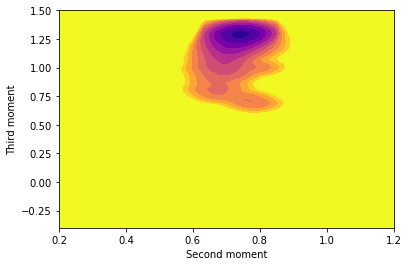
The free energy surface that you get from this calculation should look something like the figure shown on the left below. Please note that in order to fully sample configuration space and in order to get a reasonably converged estimate of the free energy you are going to have to use many more time steps than you did in previous exercises. The figure shown on the right is the free energy surface obtained if you run at a temperature of \(k_B T = 0.1 \epsilon\). As you can see a much smaller volume of configuration space is explored at this lower temperature
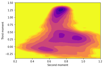 The free energy for Lennard Jones seven calculated by computing a histogram based on an MD trajectory at a temperature of 0.2 (left) and at a temperature of 0.1.
Rerun the calculation of the free energy surface at a lower temperature. What differences do you observe at the lower temperature? Why might these differences be problematic?
To learn more: Running at a lower temperature
When you run the simulation at a lower temperature you should see that the system no longer explores all the basins in the free energy landscape. If the temperature is sufficiently low the system will remain trapped in the original configuration throughout the whole simulation run. At very low temperatures this may be the correct behavior and the free energy estimate you obtain may prove to be a reasonable estimate. At the same time, however, lowering the temperature makes the barrier crossing a rarer event. It thus becomes less likely that you will observe a crossing between basins in a lower temperature simulation. The fact that the histogram shows that the probability of observing these configurations is zero may thus simply be a consequence of the fact that the simulation is not converged. The free energy will thus look like the one shown below instead of looking like the one in the previous hidden section:
 The free energy for Lennard Jones seven calculated by computing a histogram based on an MD trajectory at a temperature of 0.2 (left) and at a temperature of 0.1.
Try the following exercises if you have time and if you wish to take this exercise further:
We can use an enhanced sampling algorithm to overcome the problems that we encountered at the end of the last exercise and to more fully explore configuration space even at low temperature. In this final exercise we are thus going to perform a metadynamics simulation on our Lennard Jones cluster. In metadynamics the system is forced to explore more of configuration space by a history dependent bias that has the following functional form:
\[ V(s,t) = \sum_{\tau=0}^t w(\tau) \exp\left( -\frac{( s(t) - s(\tau))^2 }{ 2\sigma^2} \right) \]
This bias potential consists of a sum of Gaussian kernels with bandwidth \(\sigma\) that are centered at the values of the CV that the system took at previous times. The weights of the kernels in this sum are time dependent because we are going to use the well-tempered variant of metadynamics which introduces one further parameter \(\gamma = \frac{T + \Delta T}{T}\).
To run metadynamics on the Lennard Jones cluster that we have been studying in this exercise using PLUMED you would delete the lines that you used to compute the histogram from the plumed input file that we have been using thus far and you would add a line like the one shown below.
METAD ARG=__FILL__ HEIGHT=__FILL__ PACE=__FILL__ SIGMA=__FILL__ GRID_MIN=-1.5,-1.5 GRID_MAX=2.5,2.5 GRID_BIN=500,500 BIASFACTOR=5
This input should be modified to instruct PLUMED to add Gaussian kernels with a bandwidth of 0.1 in both the second and third moment of the distribution of coordination numbers and a height of 0.05 \(\epsilon\) every 50 MD steps. The metadynamics calculation should then be run using simplemd at a temperature of \(k_B T = 0.1 \epsilon\).
A nice feature of the metadynamics method is that, if the simulation is converged, the final bias potential is a related to the underlying free energy surface by:
\[ F(s) = - \frac{T + \Delta T}{\Delta T} V(s,t) \]
This formula is implemented in the tool sum_hills that is part of the PLUMED package. To run sum_hills on the output of your metadynamics simulation you can run the command:
plumed sum_hills --hills HILLS
This command should output a file called fes.dat that contains the final estimate of the free energy surface that was calculated using metadynamics.
Try to run the sum_hills command on the HILLS file output by your metadynamics simulation. Visualize the fes.dat file that is output by using gnuplot or some similar plotting package.
Try the following exercises if you have time and if you wish to take this exercise further:
This exercise has hopefully given you a sense of the sorts of calculations that can be performed using PLUMED. Hopefully you now have an understanding of how PLUMED input files are structured so that variables can be passed between different actions. Furthermore, you should have seen how PLUMED can be used both to analyze trajectories and to add in additional forces that force the system to undergo transitions that it would not otherwise undergo.
Obviously, given the short time available to us in this tutorial, we have only scratched the surface in terms of what PLUMED can be used to do and in terms of how metadynamics calculations are run in practice. If you want to understand more about how to run PLUMED we would recommend that you start by reading the chapter that we provided a link to in the introduction to this tutorial. For now though well done on completing the exercise and good luck with your future PLUMED-related endeavors.
 1.8.14