 |
|
|
| |
|
|
The aim of this tutorial is to introduce the users to the use of constant biases in PLUMED.
The TARBALL for this tutorial contains the following files:
This tutorial has been tested on a pre-release version of version 2.4. However, it should not take advantage of 2.4-only features, thus should also work with version 2.3.
PLUMED can calculate conformational properties of a system a posteriori as well as on-the-fly. This information can be use to manipulate a simulation on-the-fly. This means adding energy terms in addition to those of the original Hamiltonian. This additional energy terms are usually referred as Bias. In the following we will see how to apply a constant bias potential with PLUMED. It is preferable to run each exercise in a separate folder.
A system at temperature \( T\) samples conformations from the canonical ensemble:
\[ P(q)\propto e^{-\frac{U(q)}{k_BT}} \]
. Here \( q \) are the microscopic coordinates and \( k_B \) is the Boltzmann constant. Since \( q \) is a highly dimensional vector, it is often convenient to analyze it in terms of a few collective variables (see Trieste tutorial: Analyzing trajectories using PLUMED ). The probability distribution for a CV \( s\) is
\[ P(s)\propto \int dq e^{-\frac{U(q)}{k_BT}} \delta(s-s(q)) \]
This probability can be expressed in energy units as a free energy landscape \( F(s) \):
\[ F(s)=-k_B T \log P(s) \]
. Now we would like to modify the potential by adding a term that depends on the CV only. That is, instead of using \( U(q) \), we use \( U(q)+V(s(q))\). There are several reasons why one would like to introduce this potential. One is to avoid that the system samples some un-desired portion of the conformational space. As an example, imagine that you want to study dissociation of a complex of two molecules. If you perform a very long simulation you will be able to see association and dissociation. However, the typical time required for association will depend on the size of the simulation box. It could be thus convenient to limit the exploration to conformations where the distance between the two molecules is lower than a given threshold. This could be done by adding a bias potential on the distance between the two molecules. Another example is the simulation of a portion of a large molecule taken out from its initial context. The fragment alone could be unstable, and one might want to add additional potentials to keep the fragment in place. This could be done by adding a bias potential on some measure of the distance from the experimental structure (e.g. on root-mean-square deviation). Whatever CV we decide to bias, it is very important to recognize which is the effect of this bias and, if necessary, remove it a posteriori. The biased distribution of the CV will be
\[ P'(s)\propto \int dq e^{-\frac{U(q)+V(s(q))}{k_BT}} \delta(s-s(q))\propto e^{-\frac{V(s(q))}{k_BT}}P(s) \]
and the biased free energy landscape
\[ F'(s)=-k_B T \log P'(s)=F(s)+V(s)+C \]
Thus, the effect of a bias potential on the free energy is additive. Also notice the presence of an undetermined constant \( C \). This constant is irrelevant for what concerns free-energy differences and barriers, but will be important later when we will learn the weighted-histogram method. Obviously the last equation can be inverted so as to obtain the original, unbiased free-energy landscape from the biased one just subtracting the bias potential
\[ F(s)=F'(s)-V(s)+C \]
Additionally, one might be interested in recovering the distribution of an arbitrary observable. E.g., one could add a bias on the distance between two molecules and be willing to compute the unbiased distribution of some torsional angle. In this case there is no straightforward relationship that can be used, and one has to go back to the relationship between the microscopic probabilities:
\[ P(q)\propto P'(q) e^{\frac{V(s(q))}{k_BT}} \]
The consequence of this expression is that one can obtained any kind of unbiased information from a biased simulation just by weighting every sampled conformation with a weight
\[ w\propto e^{\frac{V(s(q))}{k_BT}} \]
That is, frames that have been explored in spite of a high (disfavoring) bias potential \( V \) will be counted more than frames that has been explored with a less disfavoring bias potential. To learn more: Summary of theory
Biased sampling
We will make use of two toy models: the first is a water dimer, i.e. two molecules of water in vacuo, that we will use to compare the effect of a constant bias on the equilibrium properties of the system that in this case can be readily computed. The second toy model is alanine dipeptide in vacuo. This system is more challenging to characterize with a standard MD simulation and we will see how we can use an interactive approach to to build a constant bias that will help in flattening the underlying free energy surface and thus sped up the sampling.
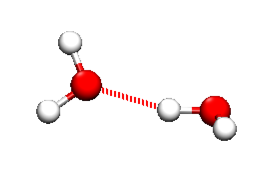
First of all let's start to learn something about the water dimer system by running a first simulations. You can start by creating a folder with the dimer.tpr file and run a simulation.
> gmx mdrun -s dimer.tpr
In this way we have a 25ns long trajectory that we can use to have a first look at the behavior of the system. Is the sampling of the relative distance between the two water molecules converged?
Use plumed driver to analyze the trajectory and evaluate the quality of the sampling.
Here you can find a sample plumed.dat file that you can use as a template. Whenever you see an highlighted FILL string, this is a string that you should replace.
# vim:ft=plumed
#compute the distance between the two oxygens
d: DISTANCE ATOMS=1,4
#accumulate block histograms
hh: HISTOGRAM ARG=d STRIDE=10 GRID_MIN=0 GRID_MAX=4.0 GRID_BIN=200 KERNEL=DISCRETE CLEAR=10000
#and dump them
DUMPGRID GRID=hh FILE=my_histogram.dat STRIDE=10000
# Print the collective variable.
PRINT ARG=d STRIDE=10 FILE=distance.dat
> plumed driver --mf_xtc traj_comp.xtc --plumed plumed.dat
> python3 do_block_histo.py > final-histo-10000.dat
If there is something you don't remember about this procedure go back and check in Trieste tutorial: Averaging, histograms and block analysis . There you can also find a python script to perform block averaging of the histograms and assess the error. The result should be comparable with the following:
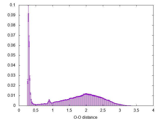
Notice the peak at 0.9 nm, this is the effect of using cut-off for the calculation of the interactions in the simulation (check the run-dimer.mdp file for the properties of the run)
Now we will try to apply a linear restraint on the relative distance and compare the resulting distribution. The new sampling will reflect the effect of the bias. Be careful about the statistics: in the simulation of exercise 1 you were post processing a trajectory of 125000 frames accumulating one frame every ten in an histogram and clearing the histogram after 10000 steps. As a result you had 12 blocks in the form of 11 analysis.* files and a final block named my_histogram.dat. In the following try to accumulate on the fly the same amount of statistics. Look into the .mdp file to see how often frames are written in a trajectory. If you write too many analysis.* files (i.e. 100 files plumed will fail with an error).
# vim:ft=plumed
#compute the distance between the two oxygens
d: DISTANCE __FILL__
#accumulate block histograms
hh: HISTOGRAM ARG=d KERNEL=DISCRETE STRIDE=500 CLEAR=500000 GRID_MIN=0 GRID_MAX=4.0 GRID_BIN=200
#and dump them
DUMPGRID __FILL__

#apply a linear restraint
lr: RESTRAINT ARG=d KAPPA=0 AT=0 SLOPE=2.5

# Print the collective variable and the bias.
PRINT __FILL__
In a new folder we can run this new simulation this time biasing and analyzing the simulation on-the-fly.
> gmx mdrun -s dimer.tpr -plumed plumed.dat
The histogram should look different.
The effect of a constant bias is that of systematically changing the probability of each conformation by a factor \( \exp(+V_{bias}/k_{B}T) \). This means that it is easily possible to recover the un-biased distribution at least in the regions of the conformational space that have been thoroughly sampled. In practice the statistical weight of each frame is not 1 anymore but is given by the exponential of the bias.
In order to recover the unbiased distribution we can post process the simulation using plumed driver to recalculate the bias felt by each frame and store this information to analyze any property. Furthermore plumed can also automatically use the bias to reweight the accumulated histogram.
# vim:ft=plumed
d: DISTANCE __FILL__

lr: RESTRAINT __FILL__
as: REWEIGHT_BIAS TEMP=298

HISTOGRAM ...
  LOGWEIGHTS=as
  ARG=d
  STRIDE=10
  GRID_MIN=0 GRID_MAX=4.0 GRID_BIN=200
  KERNEL=DISCRETE
  CLEAR=10000
... HISTOGRAM

DUMPGRID __FILL__
PRINT ARG=*.* FILE=COLVAR STRIDE=1
Be careful again about the difference in the way statistics is accumulated on-the-fly or for post processing. This is not critical for the result but is important in order to have comparable histograms, that is histograms with comparable noise. Remember to give different names to the new histogram otherwise the one obtained before will be overwritten.
> plumed driver --mf_xtc traj_comp.xtc --plumed plumed.dat
> python3 do_block_histo.py > histo-biased.dat
> python3 do_block_histo.py > histo-reweighted.dat
Now the resulting histogram should be comparable to the reference one.
Do you expect a different behavior? This time we can write the plumed input file in such a way to compare directly the biased and unbiased histograms.
# vim:ft=plumed
#calculate the distance
d: DISTANCE ATOMS=1,4
#apply the quadratic restraint centered at a distance of 0.5 nm
lr: RESTRAINT ARG=d KAPPA=10 AT=0.5
#accumulate the biased histogram
hh: HISTOGRAM ARG=d STRIDE=500 GRID_MIN=0 GRID_MAX=4.0 GRID_BIN=200 KERNEL=DISCRETE CLEAR=500000
#dumpit
DUMPGRID GRID=hh FILE=my_histogram.dat STRIDE=500000
#calculate the weights from the constant bias
as: REWEIGHT_BIAS TEMP=298
#accumulate the unbiased histogram
hhu: HISTOGRAM ARG=d STRIDE=500 GRID_MIN=0 GRID_MAX=4.0 GRID_BIN=200 KERNEL=DISCRETE CLEAR=500000 LOGWEIGHTS=as
#dumpit
DUMPGRID GRID=hhu FILE=myhistu.dat STRIDE=500000
#print distance and bias
PRINT ARG=d,lr.bias FILE=distance.dat STRIDE=50
The comparison of the two histograms with the former will show the effect of the weak quadratic bias on the simulation.
> python3 do_block_histo.py > histo-biased.dat
> python3 do_block_histo.py > histo-reweighted.dat
In the above cases we have always applied weak biases. Sometimes biases are useful to prevent the system in reaching some region of the conformational space. In this case instead of using RESTRAINT , we can make use of lower or upper restraints, e.g. LOWER_WALLS and UPPER_WALLS.
What happen to the histogram when we use walls?
# vim:ft=plumed
d: DISTANCE ATOMS=1,4
uw: UPPER_WALLS ARG=d KAPPA=1000 AT=2.5
# accumulate the biased histogram
__FILL__
#dumpit
__FILL__
# calcualte the weights from the constant bias
__FILL__
#accumulate the unbiased histogram
__FILL__
#dumpit
__FILL__
#print distance and bias
__FILL__
Run it.
> gmx mdrun -s dimer.tpr -plumed plumed.dat
If we have not sampled a region thoroughly enough it is not possible to estimate the histogram in that region even using reweighting (reweighting is not magic!).
The main issue in sampling rare events is that importance sampling algorithms spend more time in low energy regions and if two low energy regions are separated by a high energy one is unlikely for the sampling algorithm to cross the high energy region and reach the other low energy one. From this point of view an algorithm based on random sampling will work better in crossing the barrier. A particularly efficient sampling can be obtained if one would know the underlying free energy and thus use that to bias the sampling and make the sampling probability uniform in the regions of relevant interest. In this exercise we will make use of the free-energy estimate along the distance collective variable to bias the sampling of the same collective variable in the dimer simulation. To do so we will make use of a table potential applied using the Bias EXTERNAL. We first need to get a smooth estimate of the free-energy from our fist reference simulations, we will do this by accumulating a histogram with kernel functions, that is continuous function centered at the value of the accumulated point and added accumulated on the discrete representation of the histogram, see Kernel density estimation .
# vim:ft=plumed
#calculate the distance
d: DISTANCE ATOMS=1,4
#accumulate the histogram using a gaussian kernel with 0.05 nm width
hh2: HISTOGRAM ARG=d STRIDE=10 GRID_MIN=0 GRID_MAX=4.0 GRID_BIN=400 BANDWIDTH=0.05
#convert to a free energy
ff: CONVERT_TO_FES GRID=__FILL__ TEMP=__FILL__
#dump the free energy
DUMPGRID GRID=__FILL__ FILE=__FILL__
by running plumed driver on the reference trajectory we obtain a free energy estimate.
> plumed driver --mf_xtc traj_comp.xtc --plumed plumed.dat
The resulting file for the free energy should be edited in order to:
The file looks like:
#! FIELDS d ff dff_d
#! SET min_d 0
#! SET max_d 4.0
#! SET nbins_d  400
#! SET periodic_d false
0.060000 -34.9754 185.606
0.070000 -26.0117 184.362
0.080000 -20.8195 181.39
0.090000 -17.5773 176.718
where the first column is the grid spacing, the second the free energy and the third the derivative of the free energy. You can edit the file as you want, for example using the following bash lines:
grep \# ff.dat | grep -v normalisation > external.dat
grep -v \# ff.dat | awk '{print $1, -$2, -$3}' | grep -v inf >> external.dat
Furthermore edit the first line of external.dat from
#! FIELDS d ff dff_d
to
#! FIELDS d ff.bias der_d
Now we have an external potential that is the opposite of the free energy and we can use it in a new folder to bias a simulation:
# vim:ft=plumed
d: DISTANCE ATOMS=1,4
EXTERNAL ARG=d FILE=__FILL__ LABEL=ff
# accumulate the biased histogram
__FILL__
#dumpit
__FILL__
# calcualte the weights from the constant bias
__FILL__
#accumulate the unbiased histogram
__FILL__
#dumpit
__FILL__
#print distance and bias
__FILL__
Run it.
> gmx mdrun -s dimer.tpr -plumed plumed.dat
How do the biased and unbiased histograms look like? In the following we will apply this concept to sample the conformational space of a more complex system.
Alanine dipeptide is characterized by multiple minima separated by relatively high free energy barriers. Here we will explore the conformational space of alanine dipeptide using a standard MD simulation, then instead of using the free energy as an external potential we will try to fit the potential using gnuplot and add a bias using an analytical function of a collective variable with MATHEVAL and BIASVALUE .
As a first test lets run an MD and generate on-the-fly the free energy as a function of the phi and psi collective variables separately.
#SETTINGS MOLFILE=user-doc/tutorials/trieste-3/aladip/aladip.pdb
# vim:ft=plumed
MOLINFO STRUCTURE=aladip.pdb
phi: TORSION ATOMS=@phi-2
psi: TORSION ATOMS=@psi-2
hhphi: HISTOGRAM ARG=phi STRIDE=10 GRID_MIN=-pi GRID_MAX=pi GRID_BIN=600 BANDWIDTH=0.05
hhpsi: HISTOGRAM ARG=psi STRIDE=10 GRID_MIN=-pi GRID_MAX=pi GRID_BIN=600 BANDWIDTH=0.05
ffphi: CONVERT_TO_FES GRID=hhphi TEMP=298
ffpsi: CONVERT_TO_FES GRID=hhpsi TEMP=298
DUMPGRID GRID=ffphi FILE=ffphi.dat
DUMPGRID GRID=ffpsi FILE=ffpsi.dat
PRINT ARG=phi,psi FILE=colvar.dat STRIDE=10
from the colvar file it is clear that we can quickly explore two minima but that the region for positive phi is not accessible. Instead of using the opposite of the free energy as a table potential here we introduce the function MATHEVAL that allows defining complex analytical functions of collective variables, and the bias BIASVALUE that allows using any continuous function of the positions as a bias.
So first we need to fit the opposite of the free energy as a function of phi in the region explored with a periodic function, because of the gaussian like look of the minima we can fit it using the von Mises distribution. In gnuplot
>gnuplot
gnuplot>plot 'ffphi.dat' u 1:(-$2+31) w l
gnuplot>f(x)=exp(k1*cos(x-a1))+exp(k2*cos(x-a2))
gnuplot>fit [-3.:-0.6] f(x) 'ffphi.dat' u 1:(-$2+31) via k1,a1,k2,a2
gnuplot>rep f(x)
The function and the resulting parameters can be used to run a new biased simulation:
#SETTINGS MOLFILE=user-doc/tutorials/trieste-3/aladip/aladip.pdb
# vim:ft=plumed
MOLINFO STRUCTURE=aladip.pdb

phi: TORSION ATOMS=@phi-2
__FILL__

MATHEVAL ...
ARG=phi
LABEL=doubleg
FUNC=exp(__FILL)+__FILL__
PERIODIC=NO
... MATHEVAL

b: BIASVALUE ARG=__FILL__
PRINT __FILL__
It is now possible to run a second simulation and observe the new behavior. The system quickly explores a new minimum. While a quantitative estimate of the free energy difference of the old and new regions is out of the scope of the current exercise what we can do is to add a new von Mises function centered in the new minimum with a comparable height, in this way we can hope to facilitate a back and forth transition along the phi collective variable.
>gnuplot
gnuplot> ...
We can now run a third simulation where both regions are biased.
#SETTINGS MOLFILE=user-doc/tutorials/trieste-3/aladip/aladip.pdb
# vim:ft=plumed
MOLINFO STRUCTURE=aladip.pdb

phi: TORSION ATOMS=@phi-2
psi: TORSION ATOMS=@psi-2


MATHEVAL ...
ARG=phi
LABEL=tripleg
FUNC=exp(k1*cos(x-a1))+exp(k2*cos(x-a2))+exp(k3*cos(x+a3))
PERIODIC=NO
... MATHEVAL

b: BIASVALUE ARG=tripleg

__FILL__

ENDPLUMED
With this third simulation it should be possible to visit both regions as a function on the phi torsion. Now it is possible to reweight the sampling and obtain a better free energy estimate along phi.
#SETTINGS MOLFILE=user-doc/tutorials/trieste-3/aladip/aladip.pdb
# vim:ft=plumed
MOLINFO STRUCTURE=aladip.pdb

phi: TORSION ATOMS=@phi-2
psi: TORSION ATOMS=@psi-2

MATHEVAL ...
ARG=phi
LABEL=tripleg
FUNC=__FILL__
PERIODIC=NO
... MATHEVAL

b: BIASVALUE ARG=tripleg
as: REWEIGHT_BIAS TEMP=298
hhphi: HISTOGRAM ARG=phi STRIDE=10 GRID_MIN=-pi GRID_MAX=pi GRID_BIN=600 BANDWIDTH=0.05 LOGWEIGHTS=as
hhpsi: HISTOGRAM ARG=psi STRIDE=10 GRID_MIN=-pi GRID_MAX=pi GRID_BIN=600 BANDWIDTH=0.05 LOGWEIGHTS=as
ffphi: CONVERT_TO_FES GRID=hhphi TEMP=298
ffpsi: CONVERT_TO_FES GRID=hhpsi TEMP=298

DUMPGRID GRID=ffphi FILE=ffphi.dat
DUMPGRID GRID=ffpsi FILE=ffpsi.dat

PRINT ARG=phi,psi FILE=colvar.dat STRIDE=10
If you have time you can extend this in two-dimensions using at the same time the phi and psi collective variables.
 1.8.14