 |
|
|
| |
|
|
The aim of this tutorial is to train users to learn the syntax of complex collective variables and use them to analyze MD trajectories of realistic biological systems and bias them with metadynamics.
Once this tutorial is completed students will be able to:
The reference trajectories and input files for the exercises proposed in this tutorial can be downloaded from github using the following command:
wget https://github.com/plumed/trieste2017/raw/master/tutorial/data/tutorial_6.tgz
This tutorial has been tested on a pre-release version of version 2.4. However, it should not take advantage of 2.4-only features, thus should also work with version 2.3.
In this tutorial we propose exercises on the following biological systems:
The BARD1 complex is a hetero-dimer composed by two domains of 112 and 117 residues each. The system is represented at coarse-grained level using the MARTINI force field.
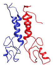
In the TARBALL of this exercise, we provide a long MD simulation of the BARD1 complex in which the two domains explore multiple different conformations.
VMD.The users are expected to:
The users are free to choose his/her favorite CVs and they are encouraged to use the on-line manual to create their own PLUMED input file. However, we encourage all the users to experiment at least with the following CVs:
1) RMSD and/or DRMSD from the native state
The following line can be added to the plumed.dat file to calculate the RMSD on the beads representing the backbone amino acids:
rmsd: RMSD REFERENCE=bard1_rmsd.pdb TYPE=OPTIMAL
while this one can be used to calculate the DRMSD between chains:
drmsd: DRMSD REFERENCE=bard1_drmsd.pdb TYPE=INTER-DRMSD LOWER_CUTOFF=0.1 UPPER_CUTOFF=1.5
2) Number of inter-chains contacts (specific, i.e. native, or all).
This can be achieved with the COORDINATION CVs, as follows:
# backbone beads index for chain A
chainA: GROUP ATOMS=1,3,5,7,9,10,12,15,17,19,21,23,25,27,29,31,33,34,36,38,41,43,45,47,49,51,53,55,57,59,61,63,66,68,70,72,74,76,79,81,83,87,89,93,95,98,102,104,106,108,111,113,115,117,119,122,125,126,128,130,132,134,136,138,140,143,145,147,149,151,154,157,159,161,163,165,167,169,172,176,178,180,182,184,186,188,190,192,195,197,199,201,202,206,208,210,212,214,215,217,219,223,224

# backbone beads index for chain B
chainB: GROUP ATOMS=226,228,230,232,234,235,238,239,240,245,246,250,252,255,256,257,259,261,264,266,268,271,273,275,278,280,282,285,287,289,291,293,295,298,300,302,304,306,308,309,310,312,314,318,320,324,326,328,330,332,334,336,338,340,342,343,345,346,348,350,352,354,358,360,362,363,368,370,372,374,376,379,381,383,386,388,390,392,394,396,398,400,402,404,406,409,411,414,416,418,420,424,426,428,430,432,434

coord: COORDINATION GROUPA=chainA GROUPB=chainB NOPBC R_0=1.0
3) A CV describing the relative orientation of the two chains.
This can be achieved, for example, by defining suitable virtual atoms with the CENTER keyword and the TORSION CV:
# virtual atom representing the first half of chain A
chainA_1: CENTER ATOMS=__FILL__
# virtual atom representing the second half of chain A
chainA_2: CENTER ATOMS=__FILL__

# virtual atom representing the first half of chain B
chainB_1: CENTER ATOMS=__FILL__
# virtual atom representing the second half of chain B
chainB_2: CENTER ATOMS=__FILL__

# torsion CV
dih: TORSION ATOMS=__FILL__
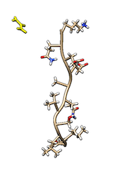
Cmyc is a small disordered peptide made of 11 amino acid. In solution, cmyc adopts a variety of different, but equally populated conformations. In the TARBALL of this exercise, we provide a long MD simulation of cmyc in presence of a single molecule of urea.
VMD.The users are expected to:
The users are free to choose his/her favorite CVs and they are encouraged to use the on-line manual to create their own PLUMED input file. However, we encourage all the users to experiment at least with the following CVs to characterize the conformational landscape of cmyc:
1) the radius of gyration of cmyc (GYRATION)
2) the content of alpha (ALPHARMSD) and beta (ANTIBETARMSD) secondary structure
The fraction of bound and unbound molecules of urea can be computed after evaluating the minimum distance among all the distances between heavy atoms of cmyc and urea, as follows:
# cmyc heavy atoms
cmyc: GROUP ATOMS=5,6,7,9,11,14,15,17,19,22,24,26,27,28,30,32,34,38,41,45,46,47,49,51,54,56,60,64,65,66,68,70,73,75,76,77,79,81,83,87,91,92,93,95,97,100,103,104,105,108,109,110,112,114,118,119,120,122,124,127,130,131,132,133,134,135,137,139,142,145,146,147,148,149,150,152,154,157,160,161,162,165,166,167,169,171,174,177,180,183,187,188

# urea heavy atoms
urea: GROUP ATOMS=192,193,194,197

# minimum distance cmyc-urea
mindist: DISTANCES GROUPA=cmyc GROUPB=urea MIN={BETA=50.}
For estimating the cmyc amino acid that bind the most and the least urea, we leave the users the choice of the best strategy.
For the calculation of ensemble averages of experimental CVs, we suggest to use:
1) 3J scalar couplings (JCOUPLING)
2) the FRET intensity between termini (FRET)
and we encourage the users to look at the examples provided in the manual for the exact syntax.
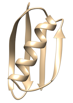
GB1 is a small protein domain with a simple beta-alpha-beta fold. It is a well studied protein that folds on the millisecond time scale. Here we use a structure based potential and well-tempered metadynamics to study the free energy of folding and unfolding. In the TARBALL of this exercise we provide the files needed to run the simulation, the user should write the plumed input file needed to bias the sampling.
The users are expected to:
The users are free to choose his/her favorite CVs and they are encouraged to use the on-line manual to create their own PLUMED input file. However, we encourage all the users to experiment at least with the following CVs to characterize the free-energy landscape of GB1:
The users should select two of them for the METAD simulation. Once you are satisfied by the convergence of your simulation, you can use one of the reweighting algorithms proposed to evaluate the free-energy difference between folded and unfolded state as a function of multiple collective variables.
#SETTINGS MOLFILE=regtest/basic/rt32/helix.pdb
#this allows you to use short-cut for dihedral angles
MOLINFO STRUCTURE=GB1_native.pdb

#add here the collective variables you want to bias

#add here the METAD bias, remember that you need to set: one SIGMA per CV, one single HEIGHT, one BIASFACTOR and one PACE.
#Using GRIDS can increase the performances, so set a as many GRID_MIN and GRID_MAX as the number of CVs with reasonable ranges
#(i.e an RMSD will range between 0 and 3, while ALPHABETA and DIHCOR will range between 0 and N of dihedrals).

#add here the printing
In summary, in this tutorial you should have learned how to use PLUMED to:
 1.8.14