 |
|
|
| |
|
|
Once this tutorial is completed students will learn to:
The tarball for this project contains the following folders:
One of the most useful target distribution is the well-tempered one. The well-tempered target distribution is [103] :
\[ p(\mathbf{s})=\frac{e^{-(\beta/\gamma) F(\mathbf{s})}}{\int d\mathbf{s} \, e^{- (\beta/\gamma) F(\mathbf{s})}} \]
where \( \gamma \) is the so-called bias factor. It is possible to show that:
\[ p(\mathbf{s}) = \frac{[ P(\mathbf{s}) ]^{1/\gamma}} {\int d\mathbf{s}\, [ P(\mathbf{s}) ]^{1/\gamma}} \]
where \( P(\mathbf{s}) \) is the unbiased distribution of CVs. Therefore the target distribution is the unbiased distribution with enhanced fluctuations and lowered barriers. This is the same distribution as sampled in well-tempered metadynamics. The advantages of this distribution are that the features of the FES (metastable states) are preserved and that the system is not forced to sample regions of high free energy as it would if we had chosen the uniform target distribution. This is specially important when biasing 2 CVs and there are large regions of very high free energy and therefore they represent un-physical configurations.
There is a caveat though, \( p(\mathbf{s}) \) depends on \( F(\mathbf{s})\) that is the function that we are trying to calculate. One way to approach this problem is to calculate \( p(\mathbf{s}) \) self-consistently [103], for instance at iteration \( k \):
\[ p^{(k+1)}(\mathbf{s})=\frac{e^{-(\beta/\gamma) F^{(k+1)}(\mathbf{s})}}{\int d\mathbf{s} \, e^{-(\beta/\gamma) F^{(k+1)}(\mathbf{s})}} \]
where:
\[ F^{(k+1)}(\mathbf{s})=-V^{(k)}(\mathbf{s}) - \frac{1}{\beta} \log p^{(k)}(\mathbf{s}) \]
Normally \( p^{(0)}(\mathbf{s}) \) is taken to be uniform. Therefore the target distribution evolves in time until it becomes stationary when the simulation has converged. It has been shown that in some cases the convergence is faster using the well-tempered target distribution than using the uniform \( p(\mathbf{s}) \) [103].
We will consider the same system employed in previous tutorials.
We consider Example 2 of the VES 1 tutorial. In that case we used a uniform target distribution that at some value decayed to zero. In this case we will use a product of two distributions:
\[ p(s)=\frac{p_{\mathrm{WT}}(s) \, p_{\mathrm{barrier}}(s)} {\int ds \, p_{\mathrm{WT}}(s) \, p_{\mathrm{barrier}}(s)} \]
where \( p_{\mathrm{WT}}(s) \) is the well-tempered target distribution and:
\[ p_{\mathrm{barrier}}(s)= \begin{cases} \frac{1}{C} \: & \mathrm{if} \: s<s_0 \\ \frac{1}{C} e^{-\frac{(s-s_0)^2}{2\sigma^2}} \: & \mathrm{if} \: s>s_0\\ \end{cases} \]
with \( C \) a normalization factor. The files needed for this exercise are in the directory Example1. This target distribution can be specified in plumed using:
td_uniform: TD_UNIFORM MINIMA=0.23 MAXIMA=0.6 SIGMA_MAXIMA=0.05
td_welltemp: TD_WELLTEMPERED BIASFACTOR=5
td_combination: TD_PRODUCT_COMBINATION DISTRIBUTIONS=td_uniform,td_welltemp

VES_LINEAR_EXPANSION ...
 ARG=d1
 BASIS_FUNCTIONS=bf1
 LABEL=b1
 TEMP=300.0
 GRID_BINS=300
 TARGET_DISTRIBUTION=td_combination
... VES_LINEAR_EXPANSION
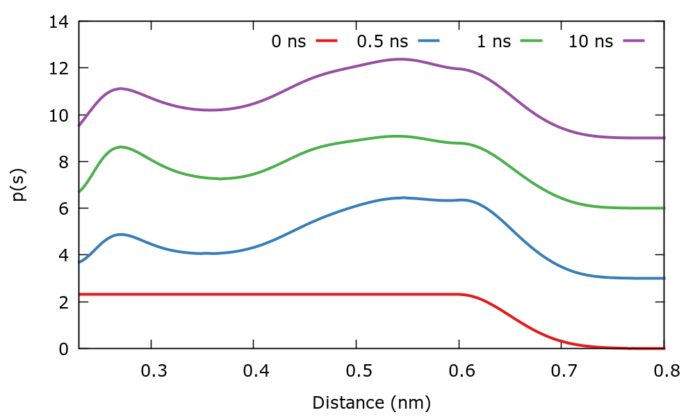
As usual, we run the example using the run.sh script. As the simulation progresses we can track the evolution of the target distribution. At variance with previous simulations where \( p(s) \) was stationary, in this case it evolves in time. The \( p(s) \) is dumped every 500 steps in a file named targetdist.b1.iter-<iteration-number>.data. You can plot these files manually or using the script plotTargetDistrib.gpi. The result should be similar to the following plot where the distribution at different times has been shifted to see more clearly the difference.
To shed some light on the nature of the well-tempered target distribution, we will compare the unbiased and biased distribution of CVs. The unbiased distribution of CVs \( P(s) \) is calculated by constructing a histogram of the CVs with weights given by:
\[ w(\mathbf{R}) \propto e^{\beta V(\mathbf{s})}. \]
The biased distribution of CVs \( p'(s) \) is calculated also by constructing a histogram of the CVs but in this case each point is assigned equal weights. The prime is added in \( p'(s) \) to distinguish the biased distribution from the target distribution \( p(s) \). If the simulation has converged then \( p'(s) = p(s) \). The files needed for this calculation are located in the Reweight directory. Since this simulation converges fast as compared to previous ones, we only disregard the first 1 ns of simulation:
sed '2,5000d' ../COLVAR > COLVAR
To calculate the biased and unbiased distribution of CVs we use the following PLUMED input:
distance:       READ FILE=COLVAR  IGNORE_TIME VALUES=d1
ves:       READ FILE=COLVAR IGNORE_TIME VALUES=b1.bias

weights: REWEIGHT_BIAS TEMP=300 ARG=ves.bias

HISTOGRAM ...
  ARG=distance
  GRID_MIN=0.23
  GRID_MAX=0.8
  GRID_BIN=301
  BANDWIDTH=0.006
  LABEL=hh1
... HISTOGRAM

HISTOGRAM ...
  ARG=distance
  GRID_MIN=0.23
  GRID_MAX=0.8
  GRID_BIN=301
  BANDWIDTH=0.006
  LOGWEIGHTS=weights
  LABEL=hh2
... HISTOGRAM

DUMPGRID GRID=hh1 FILE=histo_biased FMT=%24.16e
DUMPGRID GRID=hh2 FILE=histo_unbiased FMT=%24.16e
If you do not understand what this input does, you might want to read once again the previous tutorials. The histograms histo_biased and histo_unbiased correspond to \( p'(s) \) and \( P(s) \) , respectively. We are interested in comparing the unbiased distribution of CVs \( P(s) \) and the well-tempered distribution \( p_{\mathrm{WT}}(s)\). We know from the equations above that:
\[ p_{\mathrm{WT}}(s) \propto [ P(\mathbf{s}) ]^{1/\gamma}, \]
and also,
\[ p_{\mathrm{WT}}(s) \propto p(s)/p_{\mathrm{barrier}}(s) \propto p'(s)/p_{\mathrm{barrier}}(s) . \]
Therefore we have two ways to calculate the well-tempered target distribution. We can compare \( P(s) \) and the well-tempered target distribution calculated in two ways with the following gnuplot lines:
biasFactor=5.
invBiasFactor=1./biasFactor
pl "./histo_unbiased" u 1:(-log($2)) w l title "P(s)"
repl "./histo_unbiased" u 1:(-log($2**invBiasFactor)) w l title "[P(s)]^(1/gamma)"
repl "< paste ./histo_biased ../targetdist.b1.iter-0.data" u 1:(-log($2/$5)) w l title "Sampled p(s)"
There is also a gnuplot script plot.gpi that should do everything for you. The output should be similar to the next plot where we plot the negative logarithm of the distributions.
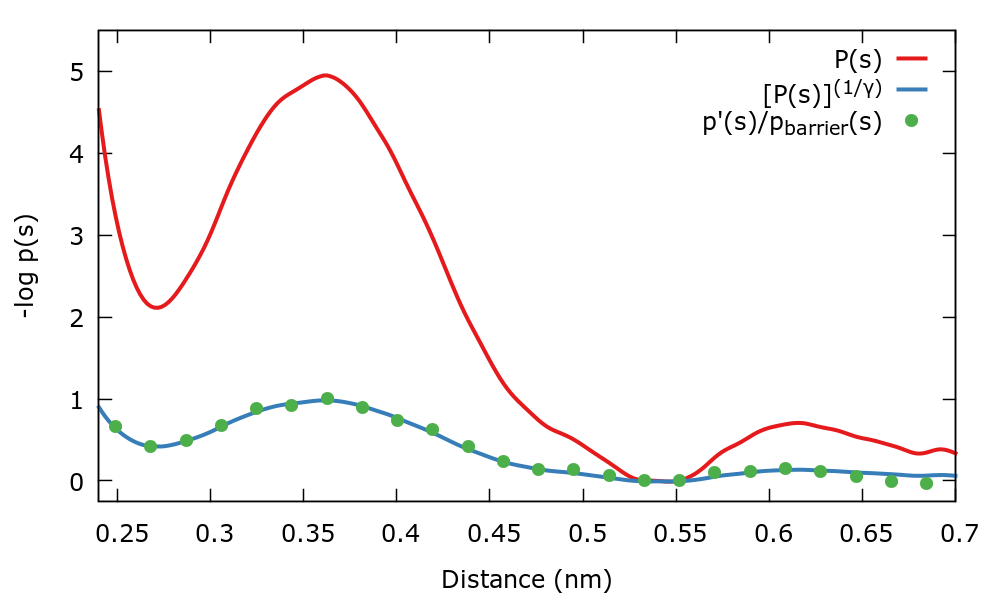
Notice that as expected both equations to calculate \( p_{\mathrm{WT}}(s)\) agree. Also the association barrier of \( 5 \: k_{\mathrm{B}} T \) becomes of \( 1 \: k_{\mathrm{B}} T \) when the well-tempered target distribution is sampled.
The take home message of this tutorial is that when the well-tempered target distribution is employed, the biased distribution of CVs preserves all the features of the unbiased distribution, but barriers are lowered. Equivalently one may say that fluctuations are enhanced.
In this example we will construct a 2 dimensional bias on the distance Na-Cl and the coordination number of Na with respect to O. The files to run this example are included in the Example2 folder. Two dimensional biases in VES can be written:
\[ V(s_1,s_2;\boldsymbol\alpha)=\sum\limits_{i_1,i_2} \alpha_{i_1,i_2} \, f_{i_1}(s_1)\, f_{i_2}(s_2) , \]
where \( f_{i_1}(s_1)\) and \( f_{i_2}(s_2) \) are the basis functions. We will choose to expand the bias potential in Legendre polynomials up to order 20 in both dimensions.
# CV1
BF_LEGENDRE ...
 ORDER=20
 MINIMUM=0.23
 MAXIMUM=0.8
 LABEL=bf1
... BF_LEGENDRE

# CV2
BF_LEGENDRE ...
 ORDER=20
 MINIMUM=2.5
 MAXIMUM=7.5
 LABEL=bf2
... BF_LEGENDRE
We have chosen the interval [0.23,0.8] nm for the distance and [2.5,7.5] for the coordination number. The total number of non-zero coefficients will be 400. In the coefficients file the indices \(i_{1}\) and \(i_{2}\) are given by the first two columns. We use the well-tempered target distribution together with a barrier at 0.6 nm on the distance Na-Cl.
td_uniform: TD_UNIFORM MINIMA=0.2,2.5 MAXIMA=0.6,7.5 SIGMA_MAXIMA=0.05,0.0
td_welltemp: TD_WELLTEMPERED BIASFACTOR=5
td_combination: TD_PRODUCT_COMBINATION DISTRIBUTIONS=td_uniform,td_welltemp

VES_LINEAR_EXPANSION ...
 ARG=d1,coord
 BASIS_FUNCTIONS=bf1,bf2
 LABEL=b1
 TEMP=300.0
 GRID_BINS=300,300
 TARGET_DISTRIBUTION=td_combination
... VES_LINEAR_EXPANSION
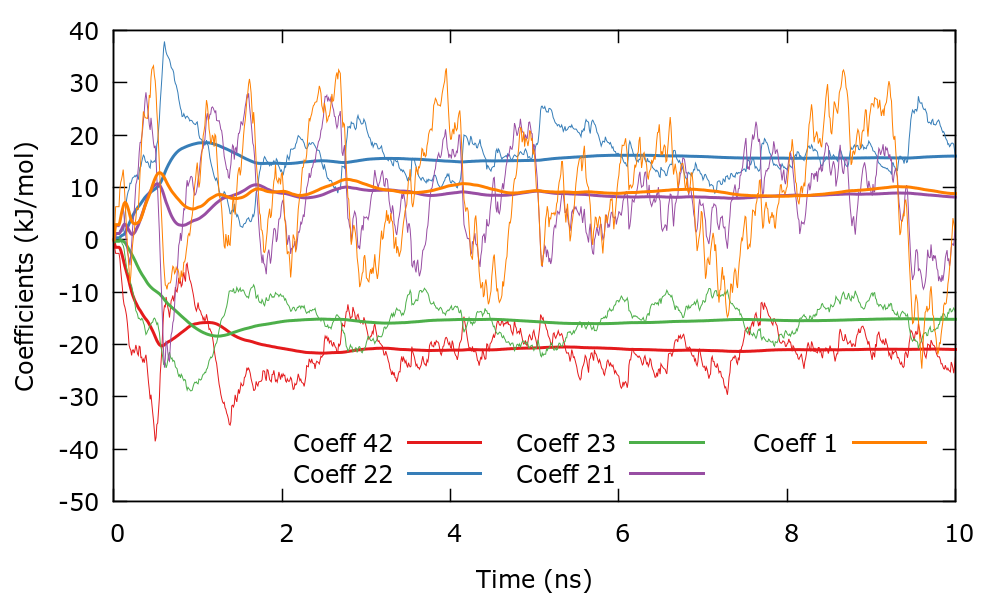
We can now run the simulation and control its progress. Since there are 400 coefficients we choose the largest (in absolute value) to control the convergence of the simulation. In this case we have chosen coefficients with indices \((i_{1},i_{2})\) as (1,0), (0,1), (1,1), (2,1), and (0,2). You can plot the evolution of the coefficients using the gnuplot script plotCoeffs.gpi. This plot should look similar to the following one. The bias therefore converges smoothly as in one dimensional problems.
The estimated FES can also be plotted to control the progress of the simulation. For instance in gnuplot,
set xr [0.23:0.7]
set yr [3:7]
set zr [0:6]
set cbr [0:6]
set pm3d map
temp=2.494
spl "./fes.b1.iter-1000.data" u 1:2:($3/temp) w pm3d notitle
There is a gnuplot script plotFes.gpi that generates the following plot for the FES after 10 ns of simulation:
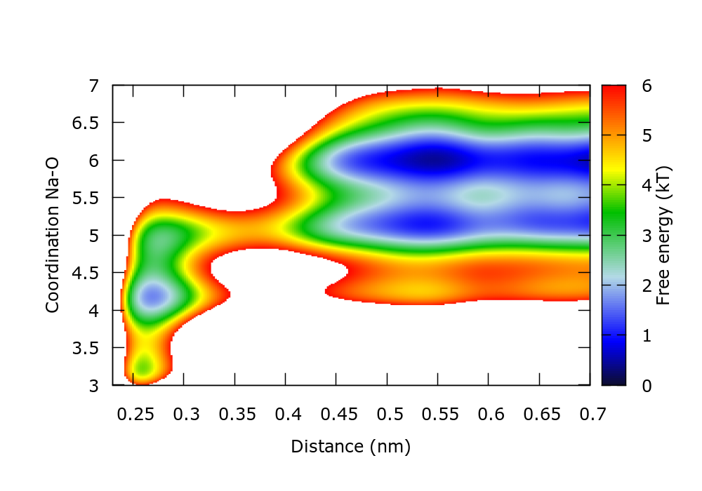
This FES agrees with that calculated through reweighting in the metadynamics tutorial.
As an exercise, you can repeat this simulation using the uniform target distribution instead of the well-tempered \( p(s) \). Compare the convergence time of both simulations. Discuss the reasons why the algorithm converges faster to the well-tempered target distribution than to the uniform one. Does it make sense to sample all the CV space uniformly?
At this point the student has acquired experience with several characteristics of the VES method. There is one tool that has proven to be instrumental for many problems and that has not yet been discussed in this series of tutorials: the use of multiple walkers. This tool will be the subject of another tutorial.
 1.8.14