 |
|
|
| |
|
|
In plumed you can bring a system in a specific state in a collective variable by means of the MOVINGRESTRAINT directive. This directive is very flexible and allows for a programmed series moving restraints. This technique can be used also to sample multiple events within a single simulation. Here I will explain the concepts of it and show some examples
Here is the tarball with the files referenced in the following .
Steered MD (SMD) is often used to drag the system from an initial configuration to a final one by pulling one or more CVs. Most of time the aim of such simulations is to prepare the system in a particular state or produce nice snapshots for a cool movie. All the CVs present in PLUMED can be used in SMD.
In SMD the Hamiltonian of the system \( H \) is modified into
\(H_\lambda\). This new Hamiltonian contains now another new term which now depends on time only via a Harmonic potential centered on a point which moves linear with time
\begin{eqnarray*} H_\lambda(X,t)&=&H(X)+U_\lambda(X,t)\\ &=&H(X)+\frac{k(t)}{2}(s(X)-\lambda(t))^2\\ &=&H(X)+\frac{k(t)}{2}(s(X)-s_0-vt)^2. \end{eqnarray*}
This means that if the \( k \) is tight enough the system will follow closely the center of the moving harmonic spring. But be careful, if the spring constant is too hard your equations of motion will now keep up since they are tuned to the fastest motion in your system so if you artificially introduce a higher frequency in your system you'll screw up the dynamics. The same is true for the pulling speed \( v \). As a matter of fact I never encountered the case where I had to lower the time step and I could all the time be happy just by making a softer spring constant or a slower steering speed. Generally, integrators of equations of motion like velocity-Verlet are very tolerant. Note that one can also make the spring constant depend on time and this, as we will see later in the examples is particularly useful to prepare your state.
In simulations, it is more convenient to adopt a situation where you specify only the starting point, the final point of collective variables and the time in which you want to cover the transition. That's why the plumed input is done in such a way.
For example, let's go back to the alanine dipeptide example encountered in The molecule of the day: alanine dipeptide. Let's say that now we want to steer from \(C_7eq \) to \( C_7ax \). If you think, just by dragging along the \( \Phi \) dihedral angle from a value of -1 to a value 1 should be enough to the state of interest. Additionally, it might be important to you not to stress the system too much, so you might want first to increase the \( k \) first so to lock the system in \( \Phi =-1 \), then move it gently to \( \Phi =1 \) and then release again your spring constant so to end up to an equilibrated and unconstrained state. This you can program in PLUMED like this
# set up two variables for Phi and Psi dihedral angles
# drag this
phi: TORSION ATOMS=5,7,9,15
# this is just to monitor that you end up in the interesting state
psi: TORSION ATOMS=7,9,15,17
# the movingrestraint
restraint: ...
        MOVINGRESTRAINT
        ARG=phi
        AT0=-1.0 STEP0=0      KAPPA0=0
        AT1=-1.0 STEP1=2000   KAPPA1=1000
        AT2=1.0  STEP2=4000   KAPPA2=1000
        AT3=1.0  STEP3=6000   KAPPA3=0
...
# monitor the two variables and various restraint outputs
PRINT STRIDE=10 ARG=* FILE=COLVAR
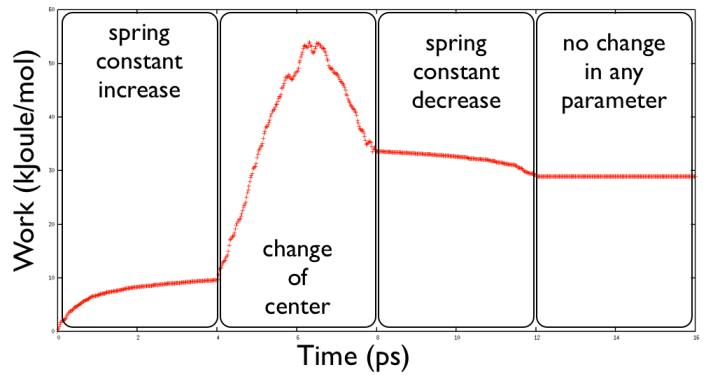
Please note the syntax of MOVINGRESTRAINT : You need one (or more) argument(s) and a set of steps denote by AT \(x\), STEP \(x\), KAPPA \(x\) where \(x\) is a incremental starting from 0 that assign the center and the harness of the spring at step STEP \(x\). What happens in between is a linear interpolation of the AT and KAPPA parameters. If those are identical in two consecutive steps then nothing is happening to that parameter. So if you put the same KAPPA and AT value in two different STEP keywords then this will give you an umbrella potential placed in the same point between the two time intervals defined by STEP. Note that you need to run a bit more than 6000 steps because after this your system has no more restraints so the actual thermalization period starts here.
The COLVAR file produced has the following shape
#! FIELDS time phi psi restraint.bias restraint.force2 restraint.phi_cntr restraint.phi_work
#! SET min_phi -pi
#! SET max_phi pi
#! SET min_psi -pi
#! SET max_psi pi
 0.000000 -1.409958 1.246193 0.000000 0.000000 -1.000000 0.000000
 0.020000 -1.432352 1.256545 0.467321 4.673211 -1.000000 0.441499
 0.040000 -1.438652 1.278405 0.962080 19.241592 -1.000000 0.918101
 0.060000 -1.388132 1.283709 1.129846 33.895372 -1.000000 1.344595
 0.080000 -1.360254 1.275045 1.297832 51.913277 -1.000000 1.691475
 ...
So we have time, phi, psi and the bias from the moving restraint. Note that at step 0 is zero since we imposed this to start from zero and ramp up in the first 2000 steps up to a value of 2000 kJ/mol/rad^2. It increases immediately since already at step 1 the harmonic potential is going to be increased in bits towards the value of 1000 which is set by KAPPA. The value of restraint.force2 is the squared force (which is a proxy of the force magnitude, despite the direction) on the CV.
\begin{eqnarray*} -\frac{\partial H_\lambda(X,t)}{\partial s}&=&-(s(X)-s_0-vt) \end{eqnarray*}
Note that the actual force on an atom of the system involved in a CV is instead
\begin{eqnarray*} -\frac{\partial H_\lambda(X,t)}{\partial x_i}&=& -\frac{\partial H_\lambda(X,t)}{\partial s} \frac{\partial s}{\partial x_i} \\ &=& -(s(X)-s_0-vt) \frac{\partial s}{\partial x_i} \end{eqnarray*}
This is important because in CVs that have a derivative that change significantly with space then you might have regions in which no force is exerted while in others you might have an enormous force on it. Typically this is the case of sigmoid functions that are used in coordination numbers in which, in the tails, they are basically flat as a function of particle positions. Additionally note that this happens on any force-based enhanced-sampling algorithm so keep it in mind. Very often people miss this aspect and complain either that a CV or a enhanced-sampling method does not work. This is another good reason to use tight spring force so to compensate in the force the lack of derivative from the CV.
The other argument in colvar is restraint.phi_cntr which is the center of the harmonic potential. This is a useful quantity so you may know how close the system is following the center of harmonic potential (more on this below). The last parameter is restraint.phi_work. The work is defined as
\begin{eqnarray*} W=\int_0^{t_s}dt\ \frac{\partial H_\lambda(t)}{\partial t} \end{eqnarray*}
so this is changing only when the Hamiltonian is changing with time. There are two time dependent contributions in this integral: one can come from the fact that \( k(t) \) changes with time and another from the fact that the center of the spring potential is changing with time.
\begin{eqnarray*} W&=&\int_0^{t_s}dt\ \frac{\partial H_\lambda(t)}{\partial t}\\ &=&\int_0^{t_s}dt\ \frac{\partial H_\lambda(t)}{\partial \lambda} \frac{\partial \lambda(t)}{\partial t} + \int_0^{t_s}dt\ \frac{\partial H_\lambda(t)}{\partial k} \frac{\partial k}{\partial t} \\ &=& \int_0^{t_s} -k(t)( s(X)-\lambda(t)) \frac{\partial \lambda(t)}{\partial t} dt + \int_0^{t_s} \frac{( s(X)-\lambda(t))^2}{2}\frac{\partial k}{\partial t} dt \\ &=& \int_0^{t_s} - k(t)( s(X)-\lambda(t)) v dt + \int_0^{t_s} \frac{( s(X)-\lambda(t))^2}{2}\frac{\partial k}{\partial t} dt \\ &\simeq& \sum_i - k(t_i)( s(X(t_i))-\lambda(t_i)) \Delta \lambda(t_i) + \sum_i\ \frac{( s(X(t_i))-\lambda(t_i))^2}{2} \Delta k(t_i) \end{eqnarray*}
where we denoted \( \Delta \lambda(t_i) \) the difference of the center of the harmonic potential respect to the step before and \( \Delta k(t_i) \) is the difference in spring constant respect to the step before. So in the exercised proposed in the first phase you see only the second part of the work since this is the part connected with the spring constant increase. After this phase you see the increase due to the motion of the center and then you later the release of the spring constant.
This you get with gnuplot:
pd@plumed:~>gnuplot
gnuplot>  p "COLVAR" u 1:7 w lp
Another couple of interesting thing that you can check is
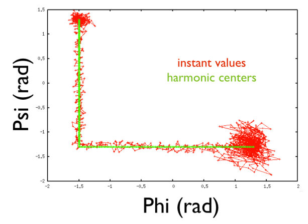
Very often it is useful to use this moving restraint to make a fancier schedule by using nice properties of MOVINGRESTRAINT. For example you can plan a schedule to drive multiple CVs at the same time in specific point of the phase space and also to stop for a while in specific using a fixed harmonic potential. This can be handy in case of an umbrella sampling run where you might want to explore a 1-dimensional landscape by acquiring some statistics in one point and then moving to the next to acquire more statistics. With MOVINGRESTRAINT you can do it in only one file. To give an example of such capabilities, let's say that we want to move from \(C7eq \) vertically toward \( \Phi =-1.5 ; \Psi=-1.3 \), stop by for a while (e.g. to acquire a statistics that you might need for an umbrella sampling), then moving toward \( \Phi =1.3 ; \Psi=-1.3 \) which roughly corresponds to \( C7ax \).
This can be programmed conveniently with MOVINGRESTRAINT by adopting the following schedule
# set up two variables for Phi and Psi dihedral angles
phi: TORSION ATOMS=5,7,9,15
psi: TORSION ATOMS=7,9,15,17
# the movingrestraint
restraint: ...
        MOVINGRESTRAINT
        ARG=phi,psi
        AT0=-1.5,1.3  STEP0=0      KAPPA0=0,0
        AT1=-1.5,1.3  STEP1=2000   KAPPA1=1000,1000
        AT2=-1.5,-1.3 STEP2=4000   KAPPA2=1000,1000
        AT3=-1.5,-1.3 STEP3=4000   KAPPA3=1000,1000
        AT4=1.3,-1.3  STEP4=6000   KAPPA4=1000,1000
        AT5=1.3,-1.3  STEP5=8000   KAPPA5=0,0
...
# monitor the two variables and various restraint outputs
PRINT STRIDE=10 ARG=* FILE=COLVAR
Note that by adding two arguments for moving restraint, now I am allowed to put two values (separated by comma, as usual for multiple values in PLUMED) and correspondingly two KAPPA values. One for each variable. Please note that no space must be used between the arguments! This is a very common fault in writing the inputs.
By plotting the instantaneous value of the variables and the value of the center of the harmonic potentials we can inspect the pathways that we make the system walk on the Ramachandran plot. (How to do this? Have a look to the header of COLVAR file to plot the right fields)
The work as we have seen is the cumulative change of the Hamiltonian in time. So it is connected with the change in energy of your system while you move it around. It has also a more important connection with the free energy via the Jarzynski equation which reads
\[ \Delta F=-\beta^{-1}\ln \langle \exp^{-\beta W} \rangle \]
This is important and says that potentially you can calculate the free energy even by driving your system very fast and out of equilibrium between two states of your interest. Unfortunately this in practice not possible since the accurate calculation of the quantity \( \langle \exp^{-\beta W} \rangle \) has a huge associated error bar since it involves the average of a noisy quantity (the work) that appears in the exponential. So, before going wild with SMD, I want to make a small exercise on how tricky that is even for the smallest system.
Now we run, say 30 SMD run and we calculate the free energy difference by using Jarzynski equality and see how this differs from the average. First note that the average \( \langle \exp^{-\beta W} \rangle \) is an average over a number of steered MD runs which start from the same value of CV and reach the final value of CV. So it is important to create initially an ensemble of states which are compatible with a given value of CVs. Let's assume that we can do this by using a restrained MD in a point (say at \( Phi=-1.5 \)). In practice the umbrella biases a bit your distribution and the best situation would be to do this with a flat bottom potential and then choosing the snapshot that correspond to the wanted starting value and start from them.
In the directory JARZ/MAKE_ENSEMBLE you find the script to run. After you generate the constrained ensemble this needs to be translated from xtc format to something that GROMACS is able to read in input, typically a more convenient gro file. To do so just to
pd@plumed:~> echo 0 | trjconv_mpi-dp-pl -f traj.xtc -s topol.tpr -o all.gro
pd@plumed:~> awk 'BEGIN{i=1}{if($1=="Generated"){outfile=sprintf("start_%d.gro",i);i++}print >>outfile; if(NF==3){close(outfile)}}' all.gro
This will generate a set of numbered gro files. Now copy them in the parallel directory MAKE_STEER. There you will find a script (script.sh) where you can set the number of runs that you want to go for. Just try 20 and let it run. Will take short time. The script will also produce a script_rama.gplt that you can use to visualize all the work performed in a single gnuplot session. Just do:
pd@plumed:~>gnuplot
gnuplot> load "script_work.gplt"
What you see is something like in Fig.
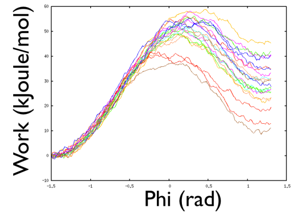
There are a number of interesting fact here. First you see that different starting points may end with very different work values. Not bad, one would say, since Jarzyinsi equality is saying that we can make an average and everything will be OK. So now calculate the average work by using the following bash one-liner:
pd@plumed:~> ntest=20; for i in `seq 1 $ntest` ; do tail -1 colvar_$i | awk '{print $7 }' ; done | awk '{g+=exp(-$1/kt) ; gg+=(exp(-$1/kt))*(exp(-$1/kt)) ; i++}END{gavg=g/i;ggavg=gg/i ; stdev=sqrt(ggavg-gavg*gavg); print "FREE ENERGY ESTIMATE ",-kt*log(gavg)," STDEV ", kt*stdev/gavg}' kt=2.4
For my test, what I get is a value of
FREE ENERGY ESTIMATE 17.482 STDEV 7.40342
and what this is saying is that the only thing that matters is the lowest work that I sampled. This has such an enormous weight over all the other trajectories that will do so that it will be the only other to count, and all the other do not matter much. So it is a kind of a waste of time. Also the standard deviation is rather high and probably it might well be that you obtain a much better result by using a standard umbrella sampling where you can use profitably most of the statistics. Here you waste most of the statistics indeed, since only the lowest work sampled will matter.
Some important point for doing some further exercises:
Targeted MD can be seen as a special case of steered MD where the RMSD from a reference structure is used as a collective variable. It can be used for example if one wants to prepare the system so that the coordinates of selected atoms are as close as possible to a target pdb structure.
As an example we can take alanine dipeptide again
# set up two variables for Phi and Psi dihedral angles
# these variables will be just monitored to see what happens
phi: TORSION ATOMS=5,7,9,15
psi: TORSION ATOMS=7,9,15,17
# creates a CV that measures the RMSD from a reference pdb structure
# the RMSD is measured after OPTIMAL alignment with the target structure
rmsd: RMSD REFERENCE=c7ax.pdb TYPE=OPTIMAL
# the movingrestraint
restraint: ...
        MOVINGRESTRAINT
        ARG=rmsd
        AT0=0.0 STEP0=0      KAPPA0=0
        AT1=0.0 STEP1=5000   KAPPA1=10000
...
# monitor the two variables and various restraint outputs
PRINT STRIDE=10 ARG=* FILE=COLVAR
(see TORSION, RMSD, MOVINGRESTRAINT, and PRINT).
Note that RMSD should be provided a reference structure in pdb format and can contain part of the system but the second column (the index) must reflect that of the full pdb so that PLUMED knows specifically which atom to drag where. The MOVINGRESTRAINT bias potential here acts on the rmsd, and the other two variables (phi and psi) are untouched. Notice that whereas the force from the restraint should be applied at every step (thus rmsd is computed at every step) the two torsion angles are computed only every 10 steps. PLUMED automatically detect which variables are used at every step, leading to better performance when complicated and computationally expensive variables are monitored - this is not the case here, since the two torsion angles are very fast to compute. Note that here the work always increase with time and never gets lower which is somewhat surprising if you think that we are moving in another metastable state. One would expect this to bend and give a signal of approaching a minimum like before. Nevertheless consider what you we are doing: we are constraining the system in one specific conformation and this is completely unnatural for a system at 300 kelvin so, even for this small system adopting a specific conformation in which all the heavy atoms are in a precise position is rather unrealistic. This means that this state is an high free energy state.
 1.8.17