 |
|
|
| |
|
|
This tutorial will show you how to you can use PLUMED to perform dimensionality reduction. The tutorial will try not to focus on the application of one particular algorithm but will instead try to show you the principles behind the implementation of these algorithms that has been adopted within PLUMED. By the end of the tutorial you will thus be able to design your own dimensionality reduction algorithm.
Once this tutorial is completed students will
The TARBALL for this project contains the following files:
In addition, you will also need to get a copy of the trajectory that we will be analyzing in this tutorial by executing the following command:
wget https://github.com/plumed/lugano2019/raw/master/handson_5/traj.dcd
The trajectory we are analyzing is a smaller version of the trajectory that was analyzed in the following paper:
In this paper the trajectory was analyzed with a variety of different dimensionality reduction algorithms and the results were compared. The paper may, therefore, be of interest.
This tutorial has been tested on v2.5 but it should also work with other versions of PLUMED.
Also notice that the .solutions direction of the tarball contains correct input files for the exercises. Please only look at these files once you have tried to solve the problems yourself. Similarly the tutorial below contains questions for you to answer that are shown in bold. You can reveal the answers to these questions by clicking on links within the tutorial but you should obviously try to answer things yourself before reading these answers.
In all of the previous tutorials we have used functions that take the position of all the atoms in the system - a \(3N\) dimensional vector, where \(N\) is the number of atoms as input. This function then outputs a single number - the value of the collective variable - that tells us where in a low dimensional space we should project that configuration. Problems can arise because this collective-variable function is many-to-one and it may thus be difficult to distinguish between every different pair of structurally distinct conformers of our system.
In this tutorial we are going to introduce an alternative approach to this business of finding collective variables. In this alternative approach we are going to stop trying to seek out a function that can take any configuration of the atoms (any \(3N\)-dimensional vector) and find its low dimensional projection on the collective variable axis. Instead we are going to take a set of configurations of the atoms (a set of \(3N\)-dimensional vectors of atom positions) and try to find a sensible set of projections for these configurations. We are going to find this low dimensional representation by seeking out an isometry between the space containing the \(3N\)-dimensional vectors of atom positions and some lower-dimensional space. This idea is explained in more detail in the following video and details on the various algorithms that we are using in the tutorial can be found in:
As you will find out if you read the chapter that is linked above there are multiple ways to construct an isometric embedding of a trajectory. This tutorial will thus try to teach you a set of basic ideas and will then encourage you to experiment and to develop your own strategy for representing the data set.
The first thing that we need to learn to do in order to run these dimensionality reduction algorithms is to store the trajectory so that we can analyze in later. The following input (once the blanks are filled in) will take the positions of the non-hydrogen atoms in our protein and store them every 1 step in an object that we can refer to later in the input using the label data. All the configurations stored in data will then be output to a pdb file once the whole trajectory is read in. Fill in the blanks in the input below now:
# This reads in the template pdb file and thus allows us to use the @nonhydrogens # special group later in the input MOLINFOSTRUCTURE=__FILL__compulsory keyword a file in pdb format containing a reference structure.MOLTYPE=protein # This stores the positions of all the nonhydrogen atoms for later analysis cc: COLLECT_FRAMEScompulsory keyword ( default=protein ) what kind of molecule is contained in the pdb file - usually not needed since protein/RNA/DNA are compatible__FILL__=@nonhydrogens # This should output the atomic positions for the frames that were collected to a pdb file called traj.pdb OUTPUT_ANALYSIS_DATA_TO_PDBcould not find this keywordUSE_OUTPUT_DATA_FROM=__FILL__use the output of the analysis performed by this object as input to your new analysis objectFILE=traj.pdbcompulsory keyword the name of the file to output to
Then, once all the blanks are filled in, run the command using:
plumed driver --mf_dcd traj.dcd
Notice that the above input stored the atomic positions of the atoms. We can use the atomic positions in many of the dimensionality reductions that will be discussed later in this tutorial or we can use a high-dimensional vector of collective variables. The following input thus gives an example of which shows you can compute and store the values the Ramachandran angles of the protein took in all the trajectory frames so that they can be analyzed using a dimensionality reduction algorithm. Try to fill in the blanks on this input and then run this form of analysis on the trajectory using the command above once more:
# This reads in the template pdb file and thus allows us to use the @nonhydrogens # special group later in the input MOLINFOSTRUCTURE=__FILL__compulsory keyword a file in pdb format containing a reference structure.MOLTYPE=protein # The following commands compute all the Ramachandran angles of the protein for you r2-phi: TORSIONcompulsory keyword ( default=protein ) what kind of molecule is contained in the pdb file - usually not needed since protein/RNA/DNA are compatibleATOMS=@phi-2 r2-psi: TORSIONthe four atoms involved in the torsional angleATOMS=@psi-2 r3-phi: TORSIONthe four atoms involved in the torsional angleATOMS=@phi-3 r3-psi: TORSIONthe four atoms involved in the torsional angleATOMS=@psi-3 r4-phi: TORSION __FILL__ r4-psi: TORSION __FILL__ r5-phi: TORSION __FILL__ r5-psi: TORSION __FILL__ r6-phi: TORSION __FILL__ r6-psi: TORSION __FILL__ r7-phi: TORSION __FILL__ r7-psi: TORSION __FILL__ r8-phi: TORSION __FILL__ r8-psi: TORSION __FILL__ r9-phi: TORSION __FILL__ r9-psi: TORSION __FILL__ r10-phi: TORSION __FILL__ r10-psi: TORSION __FILL__ r11-phi: TORSION __FILL__ r11-psi: TORSION __FILL__ r12-phi: TORSION __FILL__ r12-psi: TORSION __FILL__ r13-phi: TORSION __FILL__ r13-psi: TORSION __FILL__ r14-phi: TORSION __FILL__ r14-psi: TORSION __FILL__ r15-phi: TORSION __FILL__ r15-psi: TORSION __FILL__ r16-phi: TORSION __FILL__ r16-psi: TORSION __FILL__ # This command stores all the Ramachandran angles that were computed cc: COLLECT_FRAMESthe four atoms involved in the torsional angle__FILL__=r2-phi,r2-psi,r3-phi,r3-psi,r4-phi,r4-psi,r5-phi,r5-psi,r6-phi,r6-psi,r7-phi,r7-psi,r8-phi,r8-psi,r9-phi,r9-psi,r10-phi,r10-psi,r11-phi,r11-psi,r12-phi,r12-psi,r13-phi,r13-psi,r14-phi,r14-psi,r15-phi,r15-psi,r16-phi,r16-psi # This command outputs all the Ramachandran angles that were stored to a file called angles_data OUTPUT_ANALYSIS_DATA_TO_COLVARcould not find this keywordUSE_OUTPUT_DATA_FROM=__FILL__use the output of the analysis performed by this object as input to your new analysis objectARG=cc.*the input for this action is the scalar output from one or more other actions.FILE=angles_datacompulsory keyword the name of the file to output to
Having learned how to store data for later analysis with a dimensionality reduction algorithm lets now apply principal component analysis (PCA) upon our stored data. In principal component analysis a low dimensional projections for our trajectory are constructed by:
To perform PCA using PLUMED we are going to use the following input with the blanks filled in:
# This reads in the template pdb file and thus allows us to use the @nonhydrogens # special group later in the input MOLINFOSTRUCTURE=__FILL__compulsory keyword a file in pdb format containing a reference structure.MOLTYPE=protein # This stores the positions of all the nonhydrogen atoms for later analysis cc: COLLECT_FRAMEScompulsory keyword ( default=protein ) what kind of molecule is contained in the pdb file - usually not needed since protein/RNA/DNA are compatible__FILL__=@nonhydrogens # This diagonalizes the covariance matrix pca: PCAcould not find this keywordUSE_OUTPUT_DATA_FROM=__FILL__use the output of the analysis performed by this object as input to your new analysis objectMETRIC=OPTIMALcompulsory keyword ( default=EUCLIDEAN ) the method that you are going to use to measure the distances between pointsNLOW_DIM=2 # This projects each of the trajectory frames onto the low dimensional space that was # identified by the PCA command dat: PROJECT_ALL_ANALYSIS_DATAcompulsory keyword number of low-dimensional coordinates requiredUSE_OUTPUT_DATA_FROM=__FILL__use the output of the analysis performed by this object as input to your new analysis objectPROJECTION=__FILL__ # This should output the atomic positions for the frames that were collected and analyzed using PCA OUTPUT_ANALYSIS_DATA_TO_PDBcompulsory keyword the projection that you wish to generate out-of-sample projections withUSE_OUTPUT_DATA_FROM=__FILL__use the output of the analysis performed by this object as input to your new analysis objectFILE=traj.pdb # This should output the PCA projections of all the coordinates OUTPUT_ANALYSIS_DATA_TO_COLVARcompulsory keyword the name of the file to output toUSE_OUTPUT_DATA_FROM=__FILL__use the output of the analysis performed by this object as input to your new analysis objectARG=dat.*the input for this action is the scalar output from one or more other actions.FILE=pca_data # These next three commands calculate the secondary structure variables. These # variables measure how much of the structure resembles an alpha helix, an antiparallel beta sheet # and a parallel beta sheet. Configurations that have different secondary structures should be projected # in different parts of the low dimensional space. alpha: ALPHARMSDcompulsory keyword the name of the file to output toRESIDUES=all abeta: ANTIBETARMSDthis command is used to specify the set of residues that could conceivably form part of the secondary structure.RESIDUES=allthis command is used to specify the set of residues that could conceivably form part of the secondary structure.STRANDS_CUTOFF=1.0 pbeta: PARABETARMSDIf in a segment of protein the two strands are further apart then the calculation of the actual RMSD is skipped as the structure is very far from being beta-sheet like.RESIDUES=allthis command is used to specify the set of residues that could conceivably form part of the secondary structure.STRANDS_CUTOFF=1.0 # These commands collect and output the secondary structure variables so that we can use this information to # determine how good our projection of the trajectory data is. cc2: COLLECT_FRAMESIf in a segment of protein the two strands are further apart then the calculation of the actual RMSD is skipped as the structure is very far from being beta-sheet like.ARG=alpha,abeta,pbeta OUTPUT_ANALYSIS_DATA_TO_COLVARthe input for this action is the scalar output from one or more other actions.USE_OUTPUT_DATA_FROM=cc2use the output of the analysis performed by this object as input to your new analysis objectARG=cc2.*the input for this action is the scalar output from one or more other actions.FILE=secondary_structure_datacompulsory keyword the name of the file to output to
To generate the projection you run the command:
plumed driver --mf_dcd traj.dcd
I would recommend visualizing this data using the GISMO plugin to VMD. You can find instructions on how to compile this code on the page below:
http://epfl-cosmo.github.io/sketchmap/index.html?page=code
(you don't need to compile the sketch-map code) Once GISMO is installed you should have an option to open it when you open vmd. The option to open GISMO can be found under Extensions>Analysis>GISMO. To visualize the results from what we have just done you should need to follow the following instructions:
If you follow the instructions above you should get an image like the one shown below:
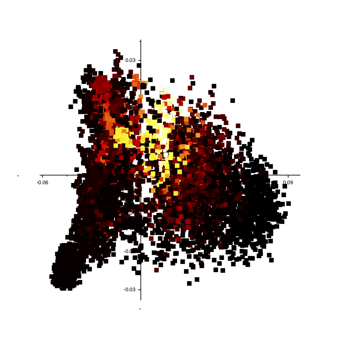
You can click on the various points in the plot and VMD will show you the structure in the corresponding trajectory frame. Furthermore, you can get a particularly useful representation of the structures by adding the following text to your ~/.vmdrc file:
user add key m {
  puts "Automatic update of secondary structure, and alignment to first frame"
  trace variable vmd_frame w structure_trace
  rmsdtt
  rmsdtt::doAlign
  destroy $::rmsdtt::w
  clear_reps top
  mol color Structure
  mol selection backbone
  mol representation NewCartoon
  mol addrep top
}
With this text in your ~/.vmdrc file VMD will align all the structures with the first frame and then show the cartoon representation of each structure when you press the m button on your keyboard
In the previous section we performed PCA on the atomic positions directly. In the section before last, however, we also saw how we can store high-dimensional vectors of collective variables and then use these vectors as input to a dimensionality reduction algorithm. We might legitimately ask, therefore, if we can do PCA using these high-dimensional vectors as input rather than atomic positions. The answer to this question is yes as long as the CV is not periodic. If any of our CVs are not periodic we cannot analyze them using the PCA action. We can, however, formulate the PCA algorithm in a different way. In this alternative formulation, which is known as classical multidimensional scaling (MDS) we do the following:
This method is used less often the PCA as the matrix that we have to diagonalize here in the third step can be considerably larger than the matrix that we have to diagonalize when we perform PCA. In fact in order to avoid this expensive diagonalization step we often select a subset of so called landmark points on which to run the algorithm directly. Projections for the remaining points are then found by using a so-called out-of-sample procedure. This is what has been done in the following input:
THISreadscould not find this keywordincould not find this keywordthecould not find this keywordtemplatecould not find this keywordpdbcould not find this keywordfilecould not find this keywordandcould not find this keywordthuscould not find this keywordallowscould not find this keyworduscould not find this keywordtocould not find this keywordusecould not find this keywordthecould not find this keyword@nonhydrogens# special group later in the input MOLINFOcould not find this keywordSTRUCTURE=beta-hairpin.pdbcompulsory keyword a file in pdb format containing a reference structure.MOLTYPE=protein # This stores the positions of all the nonhydrogen atoms for later analysis cc: COLLECT_FRAMEScompulsory keyword ( default=protein ) what kind of molecule is contained in the pdb file - usually not needed since protein/RNA/DNA are compatibleATOMS=@nonhydrogens # This should output the atomic positions for the frames that were collected and analyzed using MDS OUTPUT_ANALYSIS_DATA_TO_PDBthe atoms whose positions we are tracking for the purpose of analyzing the dataUSE_OUTPUT_DATA_FROM=ccuse the output of the analysis performed by this object as input to your new analysis objectFILE=traj.pdb # The following commands compute all the Ramachandran angles of the protein for you r2-phi: TORSIONcompulsory keyword the name of the file to output toATOMS=@phi-2 r2-psi: TORSIONthe four atoms involved in the torsional angleATOMS=@psi-2 r3-phi: TORSIONthe four atoms involved in the torsional angleATOMS=@phi-3 r3-psi: TORSIONthe four atoms involved in the torsional angleATOMS=@psi-3 r4-phi: TORSION __FILL__ r4-psi: TORSION __FILL__ r5-phi: TORSION __FILL__ r5-psi: TORSION __FILL__ r6-phi: TORSION __FILL__ r6-psi: TORSION __FILL__ r7-phi: TORSION __FILL__ r7-psi: TORSION __FILL__ r8-phi: TORSION __FILL__ r8-psi: TORSION __FILL__ r9-phi: TORSION __FILL__ r9-psi: TORSION __FILL__ r10-phi: TORSION __FILL__ r10-psi: TORSION __FILL__ r11-phi: TORSION __FILL__ r11-psi: TORSION __FILL__ r12-phi: TORSION __FILL__ r12-psi: TORSION __FILL__ r13-phi: TORSION __FILL__ r13-psi: TORSION __FILL__ r14-phi: TORSION __FILL__ r14-psi: TORSION __FILL__ r15-phi: TORSION __FILL__ r15-psi: TORSION __FILL__ r16-phi: TORSION __FILL__ r16-psi: TORSION __FILL__ # This command stores all the Ramachandran angles that were computed angles: COLLECT_FRAMESthe four atoms involved in the torsional angle__FILL__=r2-phi,r2-psi,r3-phi,r3-psi,r4-phi,r4-psi,r5-phi,r5-psi,r6-phi,r6-psi,r7-phi,r7-psi,r8-phi,r8-psi,r9-phi,r9-psi,r10-phi,r10-psi,r11-phi,r11-psi,r12-phi,r12-psi,r13-phi,r13-psi,r14-phi,r14-psi,r15-phi,r15-psi,r16-phi,r16-psi # Lets now compute the matrix of distances between the frames in the space of the Ramachandran angles distmat: EUCLIDEAN_DISSIMILARITIEScould not find this keywordUSE_OUTPUT_DATA_FROM=__FILL__use the output of the analysis performed by this object as input to your new analysis objectMETRIC=EUCLIDEAN # Now select 500 landmark points to analyze fps: LANDMARK_SELECT_FPScompulsory keyword ( default=EUCLIDEAN ) the method that you are going to use to measure the distances between pointsUSE_OUTPUT_DATA_FROM=__FILL__use the output of the analysis performed by this object as input to your new analysis objectNLANDMARKS=500 # Run MDS on the landmarks mds: CLASSICAL_MDScompulsory keyword the number of landmarks that you would like to select__FILL__=fpscould not find this keywordNLOW_DIM=2 # Project the remaining trajectory data osample: PROJECT_ALL_ANALYSIS_DATAcompulsory keyword number of low-dimensional coordinates requiredUSE_OUTPUT_DATA_FROM=__FILL__use the output of the analysis performed by this object as input to your new analysis objectPROJECTION=__FILL__ # This command outputs all the projections of all the points in the low dimensional space OUTPUT_ANALYSIS_DATA_TO_COLVARcompulsory keyword the projection that you wish to generate out-of-sample projections withUSE_OUTPUT_DATA_FROM=__FILL__use the output of the analysis performed by this object as input to your new analysis objectARG=osample.*the input for this action is the scalar output from one or more other actions.FILE=mds_data # These next three commands calculate the secondary structure variables. These # variables measure how much of the structure resembles an alpha helix, an antiparallel beta sheet # and a parallel beta sheet. Configurations that have different secondary structures should be projected # in different parts of the low dimensional space. alpha: ALPHARMSDcompulsory keyword the name of the file to output toRESIDUES=all abeta: ANTIBETARMSDthis command is used to specify the set of residues that could conceivably form part of the secondary structure.RESIDUES=allthis command is used to specify the set of residues that could conceivably form part of the secondary structure.STRANDS_CUTOFF=1.0 pbeta: PARABETARMSDIf in a segment of protein the two strands are further apart then the calculation of the actual RMSD is skipped as the structure is very far from being beta-sheet like.RESIDUES=allthis command is used to specify the set of residues that could conceivably form part of the secondary structure.STRANDS_CUTOFF=1.0 # These commands collect and output the secondary structure variables so that we can use this information to # determine how good our projection of the trajectory data is. cc2: COLLECT_FRAMESIf in a segment of protein the two strands are further apart then the calculation of the actual RMSD is skipped as the structure is very far from being beta-sheet like.ARG=alpha,abeta,pbeta OUTPUT_ANALYSIS_DATA_TO_COLVARthe input for this action is the scalar output from one or more other actions.USE_OUTPUT_DATA_FROM=cc2use the output of the analysis performed by this object as input to your new analysis objectARG=cc2.*the input for this action is the scalar output from one or more other actions.FILE=secondary_structure_datacompulsory keyword the name of the file to output to
This input collects all the torsional angles for the configurations in the trajectory. Then, at the end of the calculation, the matrix of distances between these points is computed and a set of landmark points is selected using a method known as farthest point sampling. A matrix that contains only those distances between the landmarks is then constructed and diagonalized by the CLASSICAL_MDS action so that projections of the landmarks can be constructed. The final step is then to project the remainder of the trajectory using the PROJECT_ALL_ANALYSIS_DATA action. Try to fill in the blanks in the input above and run this calculation now using the command:
plumed driver --mf_dcd traj.dcd
Once the calculation has completed you can, once again, visualize the data generated using the GISMO plugin.
The two algorithms (PCA and MDS) that we have looked at thus far are both linear dimensionality reduction algorithms. In addition to these there are a whole class of non-linear dimensionality reduction reduction algorithms which work by transforming the matrix of dissimilarities between configurations, calculating geodesic rather than Euclidean distances between configurations or by changing the form of the loss function that is optimized. In this final exercise we are going to use an algorithm that uses the last of the these three strategies to construct a non-linear projection. The algorithm is known as sketch-map and an input for sketch-map is provided below:
# This reads in the template pdb file and thus allows us to use the @nonhydrogens # special group later in the input MOLINFOSTRUCTURE=__FILL__compulsory keyword a file in pdb format containing a reference structure.MOLTYPE=protein # This stores the positions of all the nonhydrogen atoms for later analysis cc: COLLECT_FRAMEScompulsory keyword ( default=protein ) what kind of molecule is contained in the pdb file - usually not needed since protein/RNA/DNA are compatible__FILL__=@nonhydrogens # This should output the atomic positions for the frames that were collected and analyzed using MDS OUTPUT_ANALYSIS_DATA_TO_PDBcould not find this keywordUSE_OUTPUT_DATA_FROM=__FILL__use the output of the analysis performed by this object as input to your new analysis objectFILE=traj.pdb # The following commands compute all the Ramachandran angles of the protein for you r2-phi: TORSIONcompulsory keyword the name of the file to output toATOMS=@phi-2 r2-psi: TORSIONthe four atoms involved in the torsional angleATOMS=@psi-2 r3-phi: TORSIONthe four atoms involved in the torsional angleATOMS=@phi-3 r3-psi: TORSIONthe four atoms involved in the torsional angleATOMS=@psi-3 r4-phi: TORSION __FILL__ r4-psi: TORSION __FILL__ r5-phi: TORSION __FILL__ r5-psi: TORSION __FILL__ r6-phi: TORSION __FILL__ r6-psi: TORSION __FILL__ r7-phi: TORSION __FILL__ r7-psi: TORSION __FILL__ r8-phi: TORSION __FILL__ r8-psi: TORSION __FILL__ r9-phi: TORSION __FILL__ r9-psi: TORSION __FILL__ r10-phi: TORSION __FILL__ r10-psi: TORSION __FILL__ r11-phi: TORSION __FILL__ r11-psi: TORSION __FILL__ r12-phi: TORSION __FILL__ r12-psi: TORSION __FILL__ r13-phi: TORSION __FILL__ r13-psi: TORSION __FILL__ r14-phi: TORSION __FILL__ r14-psi: TORSION __FILL__ r15-phi: TORSION __FILL__ r15-psi: TORSION __FILL__ r16-phi: TORSION __FILL__ r16-psi: TORSION __FILL__ # This command stores all the Ramachandran angles that were computed angles: COLLECT_FRAMESthe four atoms involved in the torsional angle__FILL__=r2-phi,r2-psi,r3-phi,r3-psi,r4-phi,r4-psi,r5-phi,r5-psi,r6-phi,r6-psi,r7-phi,r7-psi,r8-phi,r8-psi,r9-phi,r9-psi,r10-phi,r10-psi,r11-phi,r11-psi,r12-phi,r12-psi,r13-phi,r13-psi,r14-phi,r14-psi,r15-phi,r15-psi,r16-phi,r16-psi # Lets now compute the matrix of distances between the frames in the space of the Ramachandran angles distmat: EUCLIDEAN_DISSIMILARITIEScould not find this keywordUSE_OUTPUT_DATA_FROM=__FILL__use the output of the analysis performed by this object as input to your new analysis objectMETRIC=EUCLIDEAN # Now select 500 landmark points to analyze fps: LANDMARK_SELECT_FPScompulsory keyword ( default=EUCLIDEAN ) the method that you are going to use to measure the distances between pointsUSE_OUTPUT_DATA_FROM=__FILL__use the output of the analysis performed by this object as input to your new analysis objectNLANDMARKS=500 # Run sketch-map on the landmarks smap: SKETCH_MAPcompulsory keyword the number of landmarks that you would like to select__FILL__=fpscould not find this keywordNLOW_DIM=2compulsory keyword the dimension of the low dimensional space in which the projections will be constructedHIGH_DIM_FUNCTION={SMAP R_0=6 A=8 B=2}compulsory keyword the parameters of the switching function in the high dimensional spaceLOW_DIM_FUNCTION={SMAP R_0=6 A=2 B=2}compulsory keyword the parameters of the switching function in the low dimensional spaceCGTOL=1E-3compulsory keyword ( default=1E-6 ) the tolerance for the conjugate gradient minimizationCGRID_SIZE=20compulsory keyword ( default=10 ) number of points to use in each grid directionFGRID_SIZE=200compulsory keyword ( default=0 ) interpolate the grid onto this number of points -- only works in 2DANNEAL_STEPS=0 # Project the remaining trajectory data osample: PROJECT_ALL_ANALYSIS_DATAcompulsory keyword ( default=10 ) the number of steps of annealing to doUSE_OUTPUT_DATA_FROM=__FILL__use the output of the analysis performed by this object as input to your new analysis objectPROJECTION=__FILL__ # This command outputs all the projections of all the points in the low dimensional space OUTPUT_ANALYSIS_DATA_TO_COLVARcompulsory keyword the projection that you wish to generate out-of-sample projections withUSE_OUTPUT_DATA_FROM=__FILL__use the output of the analysis performed by this object as input to your new analysis objectARG=osample.*the input for this action is the scalar output from one or more other actions.FILE=smap_data # These next three commands calculate the secondary structure variables. These # variables measure how much of the structure resembles an alpha helix, an antiparallel beta sheet # and a parallel beta sheet. Configurations that have different secondary structures should be projected # in different parts of the low dimensional space. alpha: ALPHARMSDcompulsory keyword the name of the file to output toRESIDUES=all abeta: ANTIBETARMSDthis command is used to specify the set of residues that could conceivably form part of the secondary structure.RESIDUES=allthis command is used to specify the set of residues that could conceivably form part of the secondary structure.STRANDS_CUTOFF=1.0 pbeta: PARABETARMSDIf in a segment of protein the two strands are further apart then the calculation of the actual RMSD is skipped as the structure is very far from being beta-sheet like.RESIDUES=allthis command is used to specify the set of residues that could conceivably form part of the secondary structure.STRANDS_CUTOFF=1.0 # These commands collect and output the secondary structure variables so that we can use this information to # determine how good our projection of the trajectory data is. cc2: COLLECT_FRAMESIf in a segment of protein the two strands are further apart then the calculation of the actual RMSD is skipped as the structure is very far from being beta-sheet like.ARG=alpha,abeta,pbeta OUTPUT_ANALYSIS_DATA_TO_COLVARthe input for this action is the scalar output from one or more other actions.USE_OUTPUT_DATA_FROM=cc2use the output of the analysis performed by this object as input to your new analysis objectARG=cc2.*the input for this action is the scalar output from one or more other actions.FILE=secondary_structure_datacompulsory keyword the name of the file to output to
This input collects all the torsional angles for the configurations in the trajectory. Then, at the end of the calculation, the matrix of distances between these points is computed and a set of landmark points is selected using a method known as farthest point sampling. A matrix that contains only those distances between the landmarks is then constructed and diagonalized by the CLASSICAL_MDS action and this set of projections is used as the initial configuration for the various minimization algorithms that are then used to optimize the sketch-map stress function. As in the previous exercise once the projections of the landmarks are found the projections for the remainder of the points in the trajectory are found by using the PROJECT_ALL_ANALYSIS_DATA action. Try to fill in the blanks in the input above and run this calculation now using the command:
plumed driver --mf_dcd traj.dcd
Once the calculation has completed you can, once again, visualize the data generated using the GISMO plugin.
This tutorial shown you that running dimensionality reduction algorithms using PLUMED involves the following stages:
There are multiple choices to be made in each of the various stages described above. For example, you can change the particular sort of data this is collected from the trajectory, there are multiple different ways to select landmarks, you can use the distances directly or you can transform them, you can use various different loss function and you can optimize the loss function using a variety of different algorithms. In this final exercise of the tutorial I thus want you to experiment with these various different choices that can be made. Use the data set that we have been working with throughout this tutorial and try to construct an interesting representation of it using some combination of Actions that we have not explored in the tutorial. Some things you can perhaps try:
 1.8.17