OPES_METAD Tutorial: Running and post-processing

Aim

The aim of this tutorial is to briefly present an example of an OPES_METAD simulation, together with some useful post-processing tools for obtaining an estimate of the free energy surface. This tutorial does not contain theory explanations. The OPES method is presented in detail in Ref. [62] and in its supporting information.

Resources

The TARBALL for this project contains the following:

• input files for running a simple double-well model with pesmd
• plumed files for OPES_METAD and METAD simulations
• FES_from_Reweighting.py: script for estimating free energy surface via reweighting
• FES_from_State.py: analogous to sum_hills, but for OPES simulations
• State_from_Kernels.py: script for obtaining an OPES state file from a kernels file

Simulating and reweighting

We will perform Langevin dynamics on the following two-dimensional model potential:

Fig. 1: Model potential

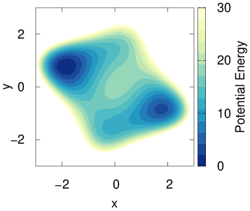
To run such simulations, we use the pesmd tool and define the potential directly inside the plumed input file.

We choose as collective variable (CV) the \(x\) coordinate only, in order to mimic a realistic situation in which some of the slow modes of the system are unknown and not accelerated by the biasing. The following is a typical plumed input for performing an OPES_METAD simulation:

Click on the labels of the actions for more information on what each action computes

UNITS 
NATURAL
( default=off ) use natural units 
 The UNITS action with label 
p: DISTANCE 
ATOMS
the pair of atom that we are calculating the distance between. 
=1,2 
COMPONENTS
( default=off ) calculate the x, y and z components of the distance separately and
store them as label.x, 
 The DISTANCE action with label p calculates the following quantities:

 Quantity   
 Description  
p.x
the x-component of the vector connecting the two atoms
p.y
the y-component of the vector connecting the two atoms
p.z
the z-component of the vector connecting the two atoms


opes: OPES_METAD 
ARG
the input for this action is the scalar output from one or more other actions. 
=p.x 
TEMP
compulsory keyword ( default=-1 )
temperature. 
=1 
PACE
compulsory keyword 
the frequency for kernel deposition 
=500 
BARRIER
compulsory keyword 
the free energy barrier to be overcome. 
=10 The OPES_METAD action with label opes calculates the following quantities:

 Quantity   
 Description  
opes.bias
the instantaneous value of the bias potential
opes.rct
estimate of \f$c(t)\f$: \f$\frac{1}{\beta}\log \langle e^{\beta V} \rangle\f$, should become flat as the simulation converges. Do NOT use for reweighting
opes.zed
estimate of \f$Z_n\f$, should become flat as no new CV-space region is explored
opes.neff
effective sample size
opes.nker
total number of compressed kernels used to represent the bias


PRINT 
FILE
the name of the file on which to output these quantities 
=COLVAR 
STRIDE
compulsory keyword ( default=1 )
the frequency with which the quantities of interest should be output 
=500 
ARG
the input for this action is the scalar output from one or more other actions. 
=p.x,p.y,opes.bias The PRINT action with label 

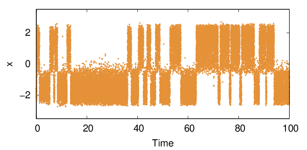
By default an OPES_METAD simulation generates a KERNELS file that, similarly to the HILLS file from METAD, contains all the Gaussians deposited during the run, and can be used for restarting a simulation. We also print a COLVAR file containing the system coordinates and the instantaneous value of the bias. Here is the time evolution of the \(x\) coordinate.

Fig. 2: Time evolution of the OPES simulation

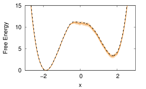
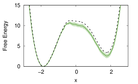
From this simulation we can estimate via reweighting the free energy surface (FES) along \(x\). We use a weighted kernel density estimation with bandwidth sigma, and use block average for uncertainty estimation. You should run the following script from the same folder where the COLVAR file is stored.

../FES_from_Reweighting.py --kt 1 --sigma 0.03 --blocks 5

As value for sigma we used the one from the last line of the KERNELS file. Notice that a similar FES estimate could have been obtained using REWEIGHT_BIAS instead of the python script. For this simple system we can compare the result with the true FES (black dashed line):

Fig. 3: Free energy estimate obtained by reweighting the OPES simulation

Note

If the COLVAR file is not available one can use instead the KERNELS file, choosing the logweight column as bias

We now run a well-tempered metadynamics simulation on the same system, to get an idea of the differences between the two methods. This is the plumed input used:

Click on the labels of the actions for more information on what each action computes

UNITS 
NATURAL
( default=off ) use natural units 
 The UNITS action with label 
p: DISTANCE 
ATOMS
the pair of atom that we are calculating the distance between. 
=1,2 
COMPONENTS
( default=off ) calculate the x, y and z components of the distance separately and
store them as label.x, 
 The DISTANCE action with label p calculates the following quantities:

 Quantity   
 Description  
p.x
the x-component of the vector connecting the two atoms
p.y
the y-component of the vector connecting the two atoms
p.z
the z-component of the vector connecting the two atoms


metad: METAD ...
   
ARG
the input for this action is the scalar output from one or more other actions. 
=p.x 
   
TEMP
the system temperature - this is only needed if you are doing well-tempered metadynamics
=1 
   
PACE
compulsory keyword 
the frequency for hill addition 
=500 
   
HEIGHT
the heights of the Gaussian hills. 
=1 
   
SIGMA
compulsory keyword 
the widths of the Gaussian hills 
=0.185815 
   
BIASFACTOR
use well tempered metadynamics and use this bias factor. 
=10 
   
GRID_MIN
the lower bounds for the grid 
=-3.5 
   
GRID_MAX
the upper bounds for the grid 
=3.5 
   
GRID_BIN
the number of bins for the grid 
=200 
   
CALC_RCT
( default=off ) calculate the \f$c(t)\f$ reweighting factor and use that to obtain
the normalized bias [rbias=bias-rct].This 
 
...The METAD action with label metad calculates the following quantities:

 Quantity   
 Description  
metad.bias
the instantaneous value of the bias potential
metad.rbias
the instantaneous value of the bias normalized using the \f$c(t)\f$ reweighting factor [rbias=bias-rct].This component can be used to obtain a reweighted histogram.
metad.rct
the reweighting factor \f$c(t)\f$.
metad.work
accumulator for work


PRINT 
FILE
the name of the file on which to output these quantities 
=COLVAR 
STRIDE
compulsory keyword ( default=1 )
the frequency with which the quantities of interest should be output 
=500 
ARG
the input for this action is the scalar output from one or more other actions. 
=p.x,p.y,metad.rbias,metad.rct The PRINT action with label 

And here is the resulting \(x\) trajectory.

Fig. 4: Time evolution of the metadynamics simulation

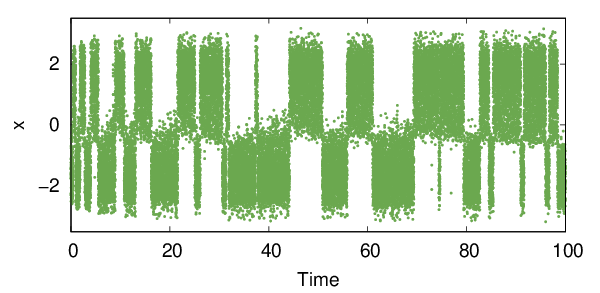
One can see that with metadynamics more transitions are present, especially in the initial part of the simulation. This is because the bias is changing quickly and can efficiently push the system through high free-energy pathways. Unfortunately, these out-of-equilibrium transitions cannot be efficiently reweighted and might lead to systematic errors.

Fig. 5: Free energy estimate obtained by (naively) reweighting the metadynamics simulation

To avoid these systematic errors, one must remove the part of the metadynamics simulation where the bias is not quasi-static. You can do so using the option --skiprows in the FES_from_Reweighting.py script. Removing an initial transient might be useful also for OPES simulations, in particular when the chosen BARRIER is much higher than the real one.

Note

Several different reweighting schemes have been proposed for metadynamics. The one we report here is among the most commonly used, but it is not guaranteed to be the most efficient.

Free energy estimate from the bias

A quick way to get a FES estimate along the biased CVs in OPES, is to directly look at the instantaneous bias \(V_t(x)\), since at convergence \(F(x)=-(1-1/\gamma)^{-1}V(x)\). For metadynamics simulations one should use the rbias instead, which is the bias shifted by the \(c(t)\) factor. In Fig. 6 we plot the COLVAR file using on the x-axis the CV \(x\) and on the y-axis this instantaneous FES estimate, \(F_t(x)\). Points are colored according to the simulation time.

Fig. 6: Free energy estimate obtained from the instantaneous bias

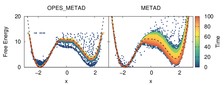
We can see that the running estimate from metadynamics has much broader oscillations. This can be seen also in Fig. 3 of Ref. [62], where only the free energy difference between the basins is plotted. It is also clearly visible that the OPES simulation does not explore free energy regions much higher than the given BARRIER parameter.

Another more common way of obtaining this direct FES estimate from the metadynamics bias is via the sum_hills tool, e.g. with the following command:

plumed sum_hills --hills HILLS --mintozero --stride 1000

An analogous procedure can be done also with OPES, starting from the STATE file printed during the simulation. This file contains the compressed kernels that are used internally to define the bias, together with all the information needed for a smooth restart. The syntax to print it is similar to the one used to print the bias grid in METAD :

Click on the labels of the actions for more information on what each action computes

UNITS 
NATURAL
( default=off ) use natural units 
 The UNITS action with label 
p: DISTANCE 
ATOMS
the pair of atom that we are calculating the distance between. 
=1,2 
COMPONENTS
( default=off ) calculate the x, y and z components of the distance separately and
store them as label.x, 
 The DISTANCE action with label p calculates the following quantities:

 Quantity   
 Description  
p.x
the x-component of the vector connecting the two atoms
p.y
the y-component of the vector connecting the two atoms
p.z
the z-component of the vector connecting the two atoms


opes: OPES_METAD ...
   
ARG
the input for this action is the scalar output from one or more other actions. 
=p.x 
   
TEMP
compulsory keyword ( default=-1 )
temperature. 
=1 
   
PACE
compulsory keyword 
the frequency for kernel deposition 
=500 
   
BARRIER
compulsory keyword 
the free energy barrier to be overcome. 
=10 
   
STATE_WFILE
write to this file the compressed kernels and all the info needed to RESTART the
simulation 
=STATE 
   
STATE_WSTRIDE
number of MD steps between writing the STATE_WFILE. 
=500*1000 
   
STORE_STATES
( default=off ) append to STATE_WFILE instead of ovewriting it each time 
 
...The OPES_METAD action with label opes calculates the following quantities:

 Quantity   
 Description  
opes.bias
the instantaneous value of the bias potential
opes.rct
estimate of \f$c(t)\f$: \f$\frac{1}{\beta}\log \langle e^{\beta V} \rangle\f$, should become flat as the simulation converges. Do NOT use for reweighting
opes.zed
estimate of \f$Z_n\f$, should become flat as no new CV-space region is explored
opes.neff
effective sample size
opes.nker
total number of compressed kernels used to represent the bias

If you did not dump the STATE file while running your simulation, you can recover it with the driver (see READ). The script State_from_Kernels.py contains the minimal input to do so, and only requires the KERNELS file.

If the STATE file is available, one can run the provided script with the following command:

../FES_from_State.py --kt 1 --all_stored

For OPES_METAD the resulting FES estimate will be very similar to the one obtained from reweighting.

In this tutorial a single simulation is presented for OPES and metadynamics, but you can check Fig. S2 and S3 in the supporting information of Ref. [62] to see the results obtained by averaging 100 independent realizations.

Some other considerations

The OPES_METAD has a few quantities one can print to monitor the simulation:

• rct, contrary to the one of METAD, converges to a constant and can be useful to quickly check the status of the simulation, especially when running with many CVs. It should not be used for reweighting.
• zed should change only when a new region of CV-space is sampled.
• neff is an estimate of the effective sample size and should always grow.
• nker is the number of compressed kernels. If it is equal to the number of deposited kernels, it means that the simulation never comes back to where it has already been (too many CVs? too small SIGMA? too small COMPRESSION_THRESHOLD?).

Finally, here are some optional keywords that might be useful:

• NLIST activates a neighbor list over the kernels. It can considerably speed up the simulation, especially when using two or more CVs.
• SIGMA_MIN can be useful to reduce the total number of compressed kernels (nker) and thus speed up the simulation. It can help especially with long simulations, and can also be added after a restart (see also FIXED_SIGMA).