 |
|
|
| |
|
|
Once this tutorial is completed students will learn to:
The tarball for this project contains the following folders:
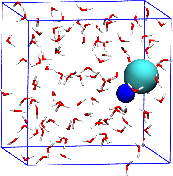
We consider the association/dissociation of NaCl in aqueous solution. The dissociation barrier is expected to be around 2.5 \(k_\mathrm{B} T\). One interesting aspect of the ion dissociation problem is that collective solvent motions play an important role in the transition. This problem has been considered in the original metadynamics paper [67] and also in reference [14] . We will use the potential developed in ref. [88] for NaCl and TIP3P water with parameters corrected to be used with long-range Coulomb solvers [96]. The system contains 1 Na, 1 Cl, and 106 water molecules (total 320 atoms).
We first perform a standard MD simulation and control the distance Na-Cl. All the files needed for this example are contained in the folder Example1 . The distance Na-Cl can be calculated in Plumed 2 using:
d1: DISTANCEATOMS=319,320the pair of atom that we are calculating the distance between.
The coordination number of Na with respect to O in water will also be calculated for later use. This variable will represent the collective motion of the solvent.
coord: COORDINATION ...GROUPA=319First list of atoms.GROUPB=1-318:3Second list of atoms (if empty, N*(N-1)/2 pairs in GROUPA are counted).SWITCH={RATIONAL R_0=0.315 D_MAX=0.5 NN=12 MM=24}This keyword is used if you want to employ an alternative to the continuous switching function defined above.NLIST( default=off ) Use a neighbor list to speed up the calculationNL_CUTOFF=0.55The cutoff for the neighbor listNL_STRIDE=10 ...The frequency with which we are updating the atoms in the neighbor list
To run LAMMPS you can use the run.sh script:
#!/bin/bash

############################################################################
# Definition of variables
############################################################################
EXE=lmp_mpi
totalCores=2
############################################################################

mpirun -np ${totalCores} ${EXE} < start.lmp > out.lmp
This command runs LAMMPS using 2 MPI threads. The use of partitions will be discussed when using multiple walkers
Once the simulation is launched, the so called COLVAR file is written. In this case it contains the following:
#! FIELDS time d1 coord
 0.200000 0.568067 5.506808
 0.400000 0.500148 4.994588
 0.600000 0.449778 4.931140
 0.800000 0.528272 5.105816
 1.000000 0.474371 5.089863
 1.200000 0.430620 5.091551
 1.400000 0.470374 4.993886
 1.600000 0.458768 4.940097
 1.800000 0.471886 4.952868
 2.000000 0.489058 4.897593
.
.
.
If you plot the time (column 1) vs the distance (column 2), for instance in gnuplot:
pl "./COLVAR" u 1:2 w lp,
you will see that the ion pair is stuck in the dissociated state during the 1 ns simulation. It is unable to cross the \(\sim5k_\mathrm{B}T\) barrier located at a distance of approximately 0.4 nm. You can also observe this behavior in the trajectory using VMD:
vmd out.dcd -psf nacl.psf
The trajectory has been saved in unwrapped format in order to avoid bonds stretching from one side to the box to the other due to periodic boundary conditions. In VMD we can wrap the atoms without breaking the bonds and show the box using the commands:
pbc wrap -compound res -all
pbc box
You can play with different visualization styles and options that VMD has. Therefore, if we want the system to go back and forth between the associated and dissociated state, we will need enhanced sampling.
We now construct a bias potential \( V(\mathbf{s}) \) on the distance Na-Cl using well-tempered metadynamics. The files for this example are contained in the directory Example2. As argument for the construction of the potential we will use the distance Na-Cl (label d1). We choose a gaussian height of 1 kJ/mol which is slightly less than 0.5 \(k_\mathrm{B} T \). The gaussian width is 0.02 nm, in the same order of the features in the FES. A rule of thumb for choosing the gaussian width is to use the standard deviation of the unbiased fluctuations of the CV. The bias factor is set to 5 since the largest barrier in the FES is expected to be roughly 5 \(k_\mathrm{B}T\). Once the metadynamics simulation is converged, the bias will be (up to an arbitrary constant):
\[ V(\mathbf{s})= - \left ( 1- \frac{1}{\gamma} \right ) F(\mathbf{s}) \]
and therefore the system will evolve under an effective free energy:
\[ \tilde{F}(\mathbf{s})=F(\mathbf{s})+V(\mathbf{s})= \frac{F(\mathbf{s})}{\gamma}, \]
that is to say, the largest barrier will be of around 1 \(k_\mathrm{B} T\). The input is:
d1: DISTANCEATOMS=319,320 metad: METAD ...the pair of atom that we are calculating the distance between.ARG=d1the input for this action is the scalar output from one or more other actions.SIGMA=0.02compulsory keyword the widths of the Gaussian hillsHEIGHT=1.the heights of the Gaussian hills.BIASFACTOR=5use well tempered metadynamics and use this bias factor.TEMP=300.0the system temperature - this is only needed if you are doing well-tempered metadynamicsPACE=500compulsory keyword the frequency for hill additionGRID_MIN=0.2the lower bounds for the gridGRID_MAX=1.0the upper bounds for the gridGRID_BIN=300the number of bins for the gridCALC_RCT...( default=off ) calculate the \f$c(t)\f$ reweighting factor and use that to obtain the normalized bias [rbias=bias-rct].This
Here the CALC_RCT keyword turns on the calculation of the time dependent constant \( c(t) \) that we will use below when reweighting the simulations.
We will also limit the exploration of the CV space by introducing an upper wall bias \( V_{wall}(\mathbf{s}) \):
\[ V_{wall}(s) = \kappa (s-s_0)^2 \mathrm{\: if \:} s>s_0 \mathrm{ \: and \: 0 \: otherwise}. \]
The wall will focus the sampling in the most interesting region of the free energy surface. The effect of this bias potential will have to be corrected later in order to calculate ensemble averages. The syntax in Plumed 2 is:
d1: DISTANCEATOMS=319,320 uwall: UPPER_WALLS ...the pair of atom that we are calculating the distance between.ARG=d1the input for this action is the scalar output from one or more other actions.AT=0.6compulsory keyword the positions of the wall.KAPPA=2000.0compulsory keyword the force constant for the wall.EXP=2compulsory keyword ( default=2.0 ) the powers for the walls.EPS=1compulsory keyword ( default=1.0 ) the values for s_i in the expression for a wallOFFSET=0. ...compulsory keyword ( default=0.0 ) the offset for the start of the wall.
You can run the simulation with the run.sh script as done in the previous example.
It is possible to try different bias factors to check the effect that it has on the trajectory and the effective FES.
In principle the cost of a metadynamics simulation should increase as the simulation progresses due to the need of adding an increasing number of Gaussian kernels to calculate the bias. However, since a grid is used to build up the bias this effect is not observed. You can check what happens if you do not use the GRID_* keywords. Remember that the bins in the grid should be small enough to describe the changes in the bias created by the Gaussian kernels. Normally a bin of size \( \sigma / 5 \) (with \( \sigma \) the gaussian width) is small enough.
One way to identify if a well tempered metadynamics simulation has converged is observing the estimated free energy surface at different times. The FES is estimated by using the relation (again up to an arbitrary constant):
\[ F(\mathbf{s}) = - \left ( \frac{\gamma}{\gamma-1} \right ) V(\mathbf{s},t) \]
and the bias potential is calculated as a sum of Gaussian kernels. This can be done with Plumed 2 using for instance:
plumed sum_hills --hills ../HILLS --min 0.1 --max 0.8 --bin 300 --stride 100
Most of the flags are self explanatory. The flag –stride 100 will result in the FES been written every 100 Gaussian kernels, i.e. 100 ps. Inside the folder FES_calculation you will find a script run.sh that executes the sum_hills command and a gnuplot script plot.gpi that can be used typing:.
gnuplot plot.gpi
After roughly 3 ns the free energy surface does not change significantly with time except for an immaterial constant \( c(t) \) that grows in time. This is in line with well-tempered metadynamics asymptotic behavior:
\[ V(\mathbf{s},t)= - \left ( 1- \frac{1}{\gamma} \right ) F(\mathbf{s}) + c(t). \]
The behavior of \( c(t) \) will be studied with greater detail later.
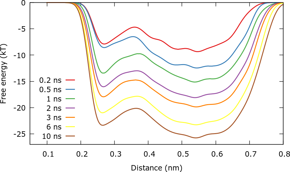
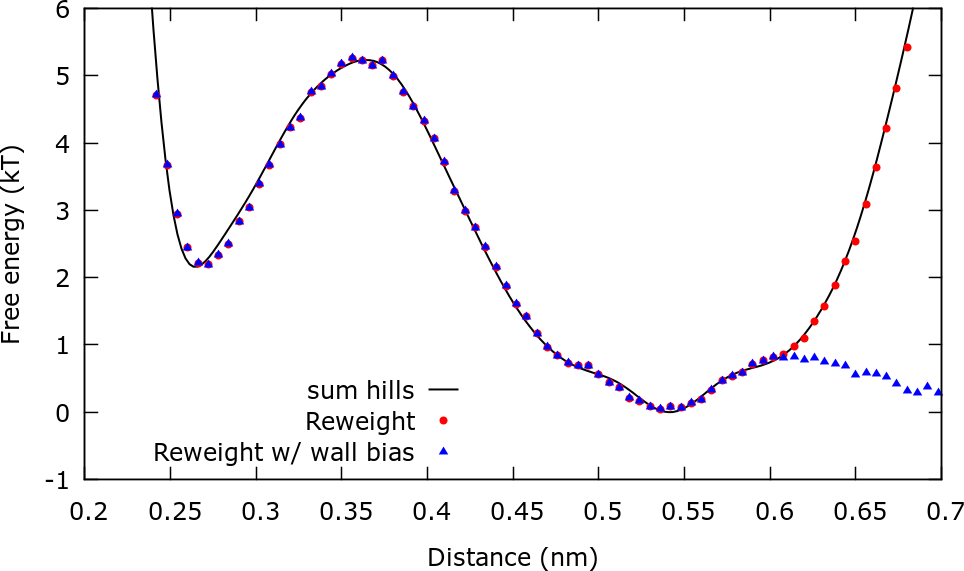
It should be stressed that we are actually not calculating the free energy \( F(\mathbf{s}) \) but rather \( F(\mathbf{s})+V_{wall}(\mathbf{s}) \). For this reason for distances higher than 0.6 nm the free energy increases sharply.
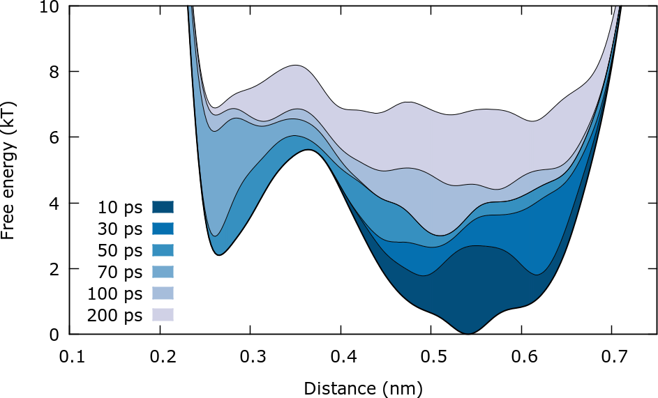
An alternative way to observe the evolution of the bias is plotting the final free energy plus the instantaneous bias. The scripts for this example can be found in the folder Bias_calculation. In this case we observe only the first 200 ps of the simulation. The (negative) bias can be calculated using:
plumed sum_hills --hills ../HILLS --min 0.1 --max 0.8 --bin 300 --stride 10 --negbias
This plot illustrates clearly how the bias is constructed to progressively "fill" the FES.
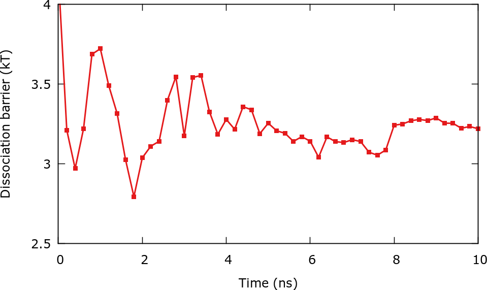
It is also possible to track convergence by controlling the evolution of some quantity connected to the free energy surface. In this case we will calculate the dissociation barrier, e.g. the height of the barrier that separates the associated state from the dissociated one. The scripts for this example are found in the folder Barrier_calculation. Using the python script calculate_barrier.py we can compute the barrier, for instance:
The script can be executed using:
python barrier_calculation.py > barrier.txt
and the results can be plotted using the gnuplot script plot.gpi. After roughly 4 ns the barrier stabilizes around 3 and 3.5 \(k_\mathrm{B} T\).
It is important to stress that it is only possible to calculate the free energy difference between two points if the system has gone back and forth between these points several times. This applies both for the calculation of a barrier and the difference in free energy between two basins. It is also important to understand that none of the free energy methods described in this series of tutorials will be able to calculate free energies of regions that have not been sampled, i.e. visited.
Reweighting the simulation on the same CV that was used for biasing can also be used as a test of convergence. We will show that in the next section.
We first reweight the simulation on the distance Na-Cl, the same CV used for biasing. This reweighting is useful to check convergence and to have an estimate of the free energy that does not rely on using kernels. For instance if some features of the FES could not be captured by the kernels, the reweighting procedure will show them. This will become clearer in the VES tutorial. The scripts to perform this calculation are found in the folder ReweightDistance. In metadynamics quasi-stationary limit the weight assigned to a given configuration is [110] :
\[ w(\mathbf{R}) \propto e^{\beta ( V(\mathbf{s},t) - c(t) )}. \]
By plotting time (column 1) versus \( c(t) \) (column 6) using the COLVAR file, the importance of taking \( c(t) \) into account becomes clear. \( c(t) \) keeps growing even after long times, reflecting the approximately rigid shift of the bias with time. Normally the first part of the trajectory is not used for reweighting since during this period the simulation has not reached the quasi-stationary limit. In this case we can discard the first 2 or 3 ns of simulation. To disregard the first 3 ns of simulation we can use sed to delete the first 15000 lines from the COLVAR file:
sed '2,15000d' ../COLVAR > COLVAR
We then use Plumed to calculate two histograms, one taking into account the wall bias and the other one neglecting it. The weights for the reweighting involving only the metadynamics bias have already been discussed while the weights considering both biases are:
\[ w(\mathbf{R}) \propto e^{\beta ( V(\mathbf{s},t) - c(t) + V_{wall}(\mathbf{s}) )}. \]
The header of the COLVAR file should be:
#! FIELDS time d1 coord metad.bias metad.rbias metad.rct metad.work uwall.bias
The input script for Plumed is:
# Read COLVAR file distance: READFILE=COLVARcompulsory keyword the name of the file from which to read these quantitiesIGNORE_TIME( default=off ) ignore the time in the colvar file.VALUES=d1 metad: READcompulsory keyword the values to read from the fileFILE=COLVARcompulsory keyword the name of the file from which to read these quantitiesIGNORE_TIME( default=off ) ignore the time in the colvar file.VALUES=metad.rbias uwall: READcompulsory keyword the values to read from the fileFILE=COLVARcompulsory keyword the name of the file from which to read these quantitiesIGNORE_TIME( default=off ) ignore the time in the colvar file.VALUES=uwall.bias # Define weights weights1: REWEIGHT_METADcompulsory keyword the values to read from the fileTEMP=300 weights2: REWEIGHT_BIASthe system temperature.TEMP=300the system temperature.ARG=metad.rbias,uwall.bias # Calculate histograms hh1: HISTOGRAM ...compulsory keyword ( default=*.bias ) the biases that must be taken into account when reweightingARG=distancethe input for this action is the scalar output from one or more other actions.GRID_MIN=0.2compulsory keyword the lower bounds for the gridGRID_MAX=0.8compulsory keyword the upper bounds for the gridGRID_BIN=100the number of bins for the gridBANDWIDTH=0.002compulsory keyword the bandwidths for kernel density estimationLOGWEIGHTS=weights1 ... hh2: HISTOGRAM ...list of actions that calculates log weights that should be used to weight configurations when calculating averagesARG=distancethe input for this action is the scalar output from one or more other actions.GRID_MIN=0.2compulsory keyword the lower bounds for the gridGRID_MAX=0.8compulsory keyword the upper bounds for the gridGRID_BIN=100the number of bins for the gridBANDWIDTH=0.002compulsory keyword the bandwidths for kernel density estimationLOGWEIGHTS=weights2 ... # Print histograms to file DUMPGRIDlist of actions that calculates log weights that should be used to weight configurations when calculating averagesGRID=hh1compulsory keyword the action that creates the grid you would like to outputFILE=histocompulsory keyword ( default=density ) the file on which to write the grid.FMT=%24.16e DUMPGRIDthe format that should be used to output real numbersGRID=hh2compulsory keyword the action that creates the grid you would like to outputFILE=histo_wallcompulsory keyword ( default=density ) the file on which to write the grid.FMT=%24.16ethe format that should be used to output real numbers
This example can be run with:
plumed --no-mpi driver --plumed plumed.dat --noatoms > plumed.out
and will generate the files histo and histo_wall. The histograms represent the probability \(p(\mathbf{s})\) of observing a given value of the CV \( \mathbf{s} \) . From the histograms the FES can be calculated using:
\[ \beta F(\mathbf{s})= - \log p(\mathbf{s}) \]
and therefore we plot the FES in gnuplot using for instance:
pl "./histo" u 1:(-log($2)) w lp
The next plot compares the estimations of the FES from sum_hills, reweighting with metadynamics bias, and reweighting using both the metadynamics bias and the upper wall bias You will find a gnuplot script plot.gpi to make this plot inside the ReweightDistance folder.
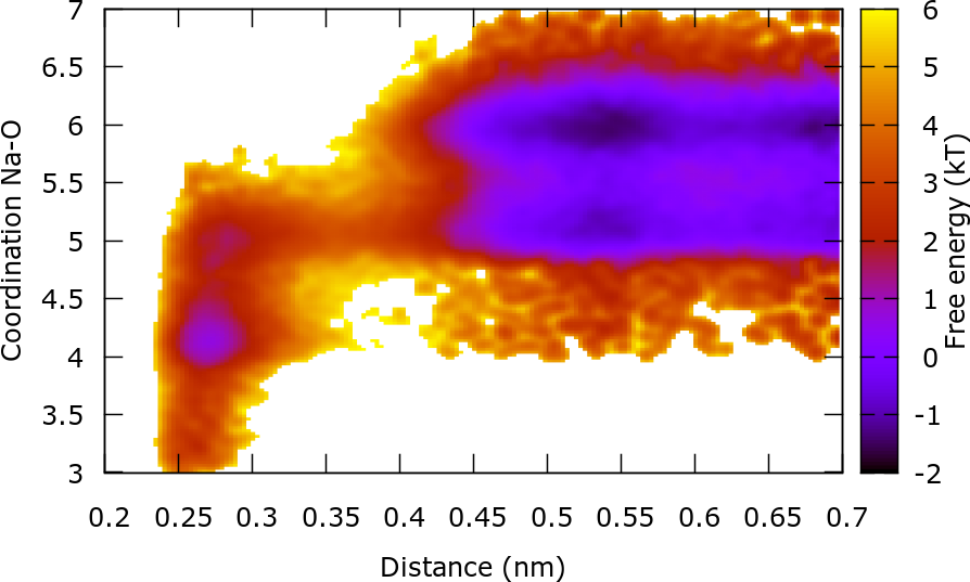
We can obtain important information of the system by reweighting on 2 CVs: The distance Na-Cl and the coordination of Na with O. This reweighting is similar to the one already done and the files that you will need are located in the ReweightBoth folder. Additionally the COLVAR file with the omitted first steps is required. The plot of the FES as a function of these 2 CVs provides important information of the association/dissociation mechanism. In the dissociated state, Na can have a coordination of 5 or 6, though it is more likely to find a coordination number of 6. However, in order to associate Na must have a coordination with O of 5. In the associated state Na can have a coordination of 3, 4 or 5. The transition state is characterized by a coordination number of ~5.
As an exercise, you can write the input files for a simulation in which a bias potential is constructed on the coordination Na-0, i.e. the solvent degree of freedom. You can use the same gaussian height as before and \( \sigma = 0.1 \).
You will find that the exploration of the CV space is not efficient. The reason is that there is a slow degree of freedom that it is not being biased: the distance Na-Cl. Furthermore you can see in the 2 CV reweighting that the coordination Na-O shows significant overlap between the associated and dissociated states.
Bear in mind that this is a rather trivial example since the existing barriers are relatively low. Real problems in materials science usually involve large barriers and are not as forgiving as this example; a bad CV may lead to huge hysteresis and problems in convergence.
We will now construct a bias potential on both CVs. We have already calculated the FES as a function of both CVs through reweighting. In this example the FES will be calculated using the metadynamics bias potential. You can use the input files from Example2.tar and changed the plumed.dat file. To construct a 2 dimensional bias with metadynamics use the following input:
__FILL__ metad: METAD ...ARG=d1,coordthe input for this action is the scalar output from one or more other actions.SIGMA=0.02,0.1compulsory keyword the widths of the Gaussian hillsHEIGHT=1.the heights of the Gaussian hills.BIASFACTOR=5use well tempered metadynamics and use this bias factor.TEMP=300.0the system temperature - this is only needed if you are doing well-tempered metadynamicsPACE=500compulsory keyword the frequency for hill additionGRID_MIN=0.15,2.the lower bounds for the gridGRID_MAX=0.9,9.the upper bounds for the gridGRID_BIN=400,400the number of bins for the gridCALC_RCT...( default=off ) calculate the \f$c(t)\f$ reweighting factor and use that to obtain the normalized bias [rbias=bias-rct].This
Once that the simulation is completed you can run plumed sum_hills to calculate the FES:
plumed sum_hills --hills HILLS --mintozero
and plot the results using the following lines in gnuplot:
set pm3d map
set zr [0:15]
spl "fes.dat" u 1:2:3
Some valuable tools for metadynamics simulations will be discussed in the VES tutorial. These include:
 1.8.17