 |
|
|
| |
|
|
This Masterclass is an introduction to the OPES (On-the-fly Probability Enhanced Sampling) method and its PLUMED implementation.
Once this Masterclass is completed, you will be able to:
We assume that you are familiar with PLUMED, metadynamics, umbrella sampling, and replica exchange. If you are not, the 2021 PLUMED Masterclass is a great place to start. In particular we suggest PLUMED Masterclass 21.1: PLUMED syntax and analysis, PLUMED Masterclass 21.3: Umbrella sampling, and PLUMED Masterclass 21.4: Metadynamics. Reading the OPES papers is also recommended [73] [74] [75].
The OPES method is an evolution of Metadynamics that also incorporates some of the ideas of the Variationally Enhanced Sampling (VES code) method. OPES is designed to be simple to use and robust with respect to suboptimal collective variables. Compared to metadynamics, it is faster in converging to a quasi-static bias and it handles multi-dimensional collective variables more efficiently.
The theory for the OPES method is presented in three separate papers [73] [74] [75]. A short overview can be found in the PLUMED documentation at OPES (On-the-fly Probability Enhanced Sampling), OPES_EXPANDED, OPES_METAD, and OPES_METAD_EXPLORE.
The OPES method aims at sampling a given target distribution over the configuration space, \(p^{\text{tg}}(\mathbf{x})\), different from the equilibrium Boltzmann distribution, \(P(\mathbf{x})\propto e^{-\beta U(\mathbf{x})}\). To do so, it iteratively builds a bias potential \(V(\mathbf{x})\), by estimating on-the-fly the needed probability distributions:
\[ V(\mathbf{x}) = -\frac{1}{\beta}\log\frac{p^{\text{tg}}(\mathbf{x})}{P(\mathbf{x})}\, . \]
The bias quickly becomes quasi-static and the desired properties, such as the free energy, can be calculated with a simple reweighting. For any given observable \(O=O(\mathbf{x})\) one can write the expectation value as:
\[ \langle O \rangle_{P} = \frac{\langle O e^{\beta V}\rangle_{p^{\text{tg}}}}{\langle e^{\beta V}\rangle_{p^{\text{tg}}}}\, . \]
There are two ways to define an OPES target distribution, a metadynamics-like and a replica-exchange-like. A replica-exchange-like target distribution is an expanded ensemble defined as a sum of overlapping probability distributions:
\[ p^{\text{tg}}_{\{\lambda\}}(\mathbf{x})=\frac{1}{N_{\{\lambda\}}}\sum_{\lambda} P_{\lambda}(\mathbf{x})\, . \]
A typical example is the temperature expanded ensemble, where each \( P_{\lambda}(\mathbf{x})\) is the same system, but at a different temperature. This kind of target distribution can be defined via a set of expansion collective variables (ECVs). The action OPES_EXPANDED can be used to sample this kind of target distributions. A metadynamics-like target distribution, is defined by its marginal over a set of collective variables (CVs), \(\mathbf{s}=\mathbf{s}(\mathbf{x})\). A typical choice for this marginal distribution is the well-tempered one:
\[ p^{\text{WT}}(\mathbf{s})=\left[P(\mathbf{s})\right]^{1/\gamma}\, , \]
where \(P(\mathbf{s})\) is the marginal over the CVs of the Boltzmann distribution, and \(\gamma>1\) is the bias factor. The well-tempered distribution is a smoother version of the original one, and in the limit of \(\gamma=\infty\) it become a uniform distribution. The actions OPES_METAD and OPES_METAD_EXPLORE can be used to sample this kind of target distributions. To learn more: Introduction to the theory
For this Masterclass we will use GROMACS 2020.6 patched with PLUMED 2.8, with the OPES module and MPI enabled. The easiest way to install all the software needed is to use the plumed-masterclass-2022 conda environment, as described here.
The data needed to complete the exercises of this Masterclass can be found on GitHub. You can clone this repository locally on your machine with the usual command:
git clone https://github.com/invemichele/masterclass-22-03.git
The repository contains all the data to run the simulations, together with the scripts to analyse them. It also contains some annotated Jupyter notebooks, that will guide us through this tutorial. Most of the information can be found there, and this page is mainly meant as an overview of the content of the notebooks.
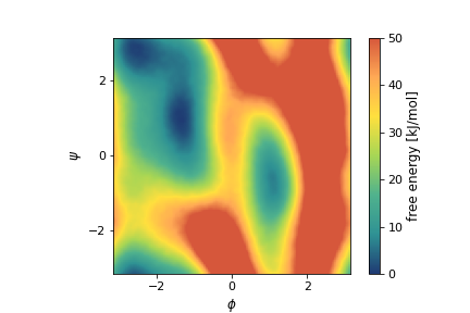
As done in some previous masterclass, we will play with a toy system, the small alanine dipeptide molecule in vacuum (ala2). It has the advantage of being a well-known system, cheap to simulate and with a higher level of complexity compared to a 2D model potential as the one used in this other OPES_METAD Tutorial: Running and post-processing. Ala2 has two main metastable basins which can be identified by a very efficient collective variable (CV), the \(\phi\) torsional angle. Here is its free energy surface (FES) as a function of the \(\phi\) and \(\psi\) angles:
We start by using OPES to sample expanded ensembles [75]. This probably is not a familiar application of adaptive-bias enhanced sampling for most of PLUMED users, so we will start with a little
The first example we consider is a multithermal simulation of alanine dipeptide. One can use replica exchange to perform a parallel tempering simulation and sample the two metastable states of alanine dipeptide, as explained for instance in Belfast tutorial: Replica exchange I. Here instead, we want to sample the same multithermal distribution not by combining simulations at different temperatures, but by adding a bias potential to a single simulation.
We choose 3 temperatures \(T_0, T_1, T_2\), ranging from 300 K to 1000 K, and setup our GROMACS simulation to run at \(T_0=300\) K. Our target distribution is then:
\[ p^{\text{tg}}(\mathbf{x})=\frac{1}{3}\left[\frac{e^{-\frac{1}{k_BT_0}U(\mathbf{x})}}{Z_0}+ \frac{e^{-\frac{1}{k_BT_1}U(\mathbf{x})}}{Z_1}+\frac{e^{-\frac{1}{k_BT_2}U(\mathbf{x})}}{Z_2}\right] \]
This can be rewritten highlighting \(P(\mathbf{x})\)
\[ p^{\text{tg}}(\mathbf{x})=P(\mathbf{x})\frac{1}{3}\left[1+ e^{-\left(\frac{1}{k_BT_1}-\frac{1}{k_BT_0}\right)U(\mathbf{x})}\frac{Z_0}{Z_1}+e^{-\left(\frac{1}{k_BT_2}-\frac{1}{k_BT_0}\right)U(\mathbf{x})}\frac{Z_0}{Z_2}\right] \]
and then using \(\Delta F_i = -k_B T_0 \log \frac{Z_i}{Z_0}\):
\[ p^{\text{tg}}(\mathbf{x})=P(\mathbf{x})\frac{1}{3}\left[1+ e^{-\frac{1-T_0/T_1}{k_BT_0}U(\mathbf{x})+\frac{1}{k_BT_0}\Delta F_1}+e^{-\frac{1-T_0/T_2}{k_BT_0}U(\mathbf{x})+\frac{1}{k_BT_0}\Delta F_2}\right] \]
so we just need to know \(\Delta F_1\) and \(\Delta F_2\), and we can sample the target multithermal distribution by using the following bias:
\[ V(U) = - k_B T_0 \log \frac{1}{3}\left[1+ e^{-\frac{1-T_0/T_1}{k_BT_0}U(\mathbf{x})+\frac{1}{k_BT_0}\Delta F_1}+e^{-\frac{1-T_0/T_2}{k_BT_0}U(\mathbf{x})+\frac{1}{k_BT_0}\Delta F_2}\right] \]
that is a function only of the potential energy \(U=U(\mathbf{x})\). In the OPES spirit, we estimate on-the-fly these free energy differences using a simple reweighting, and iteratively reach the target distribution. The final bias expression is determined by these quantities \(\frac{1-T_0/T_i}{k_BT_0}U(\mathbf{x})\), that we call expansion_cv (ECVs). There are several types of expanded ensembles that might be of interest, and in order to sample them with OPES one simply needs to find the explicit form of the corresponding ECVs. To sample the same expanded ensemble with replica exchange, one has to run a different replica of the system for each of the ECVs. To learn more: The bias that we need
Enough equations, here is the plumed input file we need to run this multithermal simulation:
ene: ENERGY ecv: ECV_MULTITHERMAL ARGcompulsory keyword the label of the internal energy of the system. =ene TEMP_MINthe minimum of the temperature range =300 TEMP_MAXthe maximum of the temperature range =1000 TEMP_STEPSthe number of steps in temperature =3 opes: OPES_EXPANDED ARGcompulsory keyword the label of the ECVs that define the expansion. =ecv.ene PACEcompulsory keyword how often the bias is updated =500
We use the OPES_EXPANDED bias action, with a multithermal expansion defined by the ECV_MULTITHERMAL action. The resulting bias is a function of the potential energy, and is updated every 500 MD steps.
In the notebook we show the shape of the resulting bias, how to check for convergence and how to reweight for estimating the free energy at different temperatures. We also explain a simple procedure that is used to automatically set a reasonable number of temperature steps, if TEMP_STEPS is not provided.
Next, we present another expanded ensemble that can also be sampled by replica exchange. We call it multiumbrella and it is composed by all the distributions sampled by a typical multiple windows umbrella sampling simulation. In this kind of umbrella sampling, one chooses a CV and runs several simulations each one with a parabolic bias potential at a different CV location (see PLUMED Masterclass 21.3: Umbrella sampling). We can use OPES to sample an expanded target distribution that is composed of all of these combined.
In multiple windows umbrella sampling, the free energy difference between the windows is estimated during postprocessing (e.g. with WHAM), in OPES this is done on-the-fly at simulation time. The main advantages are that choosing the number and location of the umbrellas becomes easier, and having a single longer simulation can also help with sampling orthogonal slow degrees of freedom.
We choose as CV the \(\phi\) angle. The ECVs we need for this type of expansion are the following:
\[ \Delta u_i = \frac{(\phi-\phi_i)^2}{2\sigma^2}\, , \]
where \(\phi_i\) are the fixed centers of the umbrellas and \(\sigma\) determines their width. Usually in umbrella sampling another parameter is used, \(k=1/\sqrt{\sigma}\), but we will see in the notebook why we made a different choice.
The plumed input we need might look like this:
phi: TORSION ATOMSthe four atoms involved in the torsional angle =5,7,9,15 ecv: ECV_UMBRELLAS_LINE ARGthe input for this action is the scalar output from one or more other actions. =phi CV_MINcompulsory keyword the minimum of the CV range to be explored =-pi CV_MAXcompulsory keyword the maximum of the CV range to be explored =pi SIGMAcompulsory keyword sigma of the umbrella Gaussians =0.2 opes: OPES_EXPANDED ARGcompulsory keyword the label of the ECVs that define the expansion. =ecv.phi PACEcompulsory keyword how often the bias is updated =500
This places umbrellas uniformly along \(\phi\), each one separated by a distance of one \(\sigma\). We can make them less close to each with the keyword SPACING. We can also provide a guess of the maximum free energy BARRIER we need to overcome, it can help speed up convergence.
In the notebook we show what kind of sampling this input provides, and invite you to play around with the parameters, to get a sense of what each option does. We also perform reweighting to obtain a FES estimate. This reweighting is done with kernel density estimation (similarly to plumed histogram function), and is interesting to see the effect of changing the bandwidth parameter.
Another advantage of using OPES to sample expanded ensembles is that it makes it very easy to combine them. We show this by running a combined multithermal and multiumbrella simulation of alanine dipeptide.
Using the multithermal expansion, we were able to sample both metastable states, but not very efficiently. With the multiumbrella target distribution we have many transitions, but we sample only at 300 K. By combining these two expansions we obtain the best of both, with frequent transitions and an efficient reweighting over a whole range of temperatures.
The drawback? We might have to deal with a lot of ECVs! However, while in a replica exchange scheme each ECV requires its own replica, with OPES we are free to use just one, or choose any number of parallel replica, in a multiple walkers scheme.
The way we combine expansions is to create a grid with all possible combinations of temperature ECVs and umbrella ECVs. So, if we have 10 ECVs for the temperature expansion and 20 for the multiumbrella one, we end up with 200 combined ECVs. This will become clearer once we look at the notebook and the simulation output.
From the point of view of the plumed input things are quite straightforward. For a combined multithermal-multiumbrella simulation it should look similar to this one:
# temperature expansion, based on energy ene: ENERGY ecv_mt: ECV_MULTITHERMAL ARGcompulsory keyword the label of the internal energy of the system. =ene TEMP_MINthe minimum of the temperature range =300 TEMP_MAXthe maximum of the temperature range =1000 # multiumbrella expansion, based on phi phi: TORSION ATOMSthe four atoms involved in the torsional angle =5,7,9,15 ecv_mu: ECV_UMBRELLAS_LINE ARGthe input for this action is the scalar output from one or more other actions. =phi CV_MINcompulsory keyword the minimum of the CV range to be explored =-pi CV_MAXcompulsory keyword the maximum of the CV range to be explored =pi SIGMAcompulsory keyword sigma of the umbrella Gaussians =0.2 # the OPES bias combines them opes: OPES_EXPANDED ARGcompulsory keyword the label of the ECVs that define the expansion. =ecv_mt.ene,ecv_mu.phi PACEcompulsory keyword how often the bias is updated =500
To fully appreciate the strength of combining these two different expansions, one can run the same simulations but using the \(\psi\) angle instead of \(\phi\), and see what happens.
We now use OPES to perform biased simulations very similar to those of metadynamics [73] [74]. We will sample a well-tempered distribution along a chosen set of collective variables.
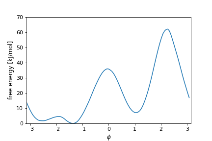
We start by biasing the \(\phi\) angle, which is known to be a good CV for alanine dipeptide. Here is how the FES along this CV looks like:
We use this simple example to get familiar with OPES_METAD, its input parameter and output quantities. We also compare it with well-tempered metadynamics, and we start to see how this two methods differ.
This also gives us the opportunity of using some of the postprocessing scripts for OPES. For OPES, there is not yet a tool similar to the sum_hills, but we can obtain the same result with simple python scripts and by dumping the state of the simulation through the STATE_WFILE keyword. This STATE file contains the compressed kernels used by OPES at a given time to represent the probability distribution, and thus the bias.
Next, we move to biasing both the Ramachandran angles of ala2. A minimal plumed input to do this is the following:
phi: TORSION ATOMSthe four atoms involved in the torsional angle =5,7,9,15 psi: TORSION ATOMSthe four atoms involved in the torsional angle =7,9,15,17 opes: OPES_METAD ARGthe input for this action is the scalar output from one or more other actions. =phi,psi PACEcompulsory keyword the frequency for kernel deposition =500 BARRIERcompulsory keyword the free energy barrier to be overcome. =40
This example gives us a nice opportunity to visualize the kernel compression algorithm in action. We can also get an idea of the differences between OPES_METAD and OPES_METAD_EXPLORE methods. The plumed inputs are identical:
phi: TORSION ATOMSthe four atoms involved in the torsional angle =5,7,9,15 psi: TORSION ATOMSthe four atoms involved in the torsional angle =7,9,15,17 opes: OPES_METAD_EXPLORE ARGthe input for this action is the scalar output from one or more other actions. =phi,psi PACEcompulsory keyword the frequency for kernel deposition =500 BARRIERcompulsory keyword the free energy barrier to be overcome. =40
From here it should be easy to compare both OPES variants to metadynamics, maybe by running some longer simulations. We can also check the way the bias converges by focusing on the estimate of the free energy difference between the basins.
In order to experiment with more than two CVs, we have to introduce a new system, alanine tetrapeptide in vacuum (ala4). It is a bigger brother of ala2, with not one but three \(\phi\) and \(\psi\) torsional angles, that can be used to sample its 8 metastable basins.
We can try to sample ala4 with each of the tree methods, METAD, OPES_METAD, and OPES_METAD_EXPLORE. How will the respective input files look like?
We run only short simulations to see how quickly the CV space is sampled by the various methods, and not for converging a FES. This example can help to appreciate the effect of the \(Z\) term in OPES_METAD. In fact, the more CVs there are, the more it plays an important role in speeding up exploration.
We can also see the effect of changing the bias factor \(\gamma\) on the sampling efficiency.
Finally, what is probably the most interesting scenario. We bias again ala2, but this time using a suboptimal collective variable. We don't know much about this CV, it could be for instance the output of a machine learning procedure. Will we be able to calculate the FES as a function of this CV? How should the plumed input files look like? Here it would be nice to also have some error bars to our estimates.
We will discuss together the results of these simulations, and also reveal how this CV was constructed.
If you prefer a more straightforward example of suboptimal CV, you can check out this OPES_METAD Tutorial: Running and post-processing.
Hopefully this masterclass helped you to start playing around with the OPES method and get a sense of what it can be useful for. If you are still interested in testing it out and understanding more about it, then you should check out the PLUMED-NEST. Just search for "opes" and you will find several papers that use the method, together with all the input files necessary to reproduce their simulations.
 1.8.17