 |
|
|
| |
|
|
This Masterclass is an introduction to the use of the SASA module of Plumed for the execution of implicit solvent simulations.
The objectives of this Masterclass are:
We assume that the person that will follow this tutorial is familiar with the Linux terminal, AMBER and basic functionality of PLUMED. Knowledge of the metadynamics enhanced sampling technique is recommended. Familiarity with gnuplot and xmgrace (or python with matplotlib) is recommended.
We will use AMBER and PLUMED to perform the calculations. Conda packages with the software required for this class have been prepared and you can install them following the instructions in this link. Make sure to install the conda package for AMBER.
If you are compiling PLUMED on your own, you will need to install the SASA module manually by adding '–enable-modules=sasa' to your './configure' command when building PLUMED.
The data needed to run the exercises of this Masterclass can be found on GitHub. You can clone this repository locally on your machine using the following command:
git clone https://github.com/andrea-arsiccio/masterclass-22-13
You will also need a python script for the calculation of free energies of transfer, available on GitHub.
The SASA module contains methods for the calculation of the solvent accessible surface area (SASA) of proteins. It can be used to include the SASA as a collective variable in metadynamics simulations, and for implicit solvent simulations.
There are two SASA functions that could be used:
SASA_HASEL: employs the algorithm described in [65] for the computation of the SASA.
SASA_LCPO: employs the algorithm described in [143] for the computation of the SASA.
The algorithm by Hasel et al. is about 2 to 3 times faster than the LCPO (linear combination of pairwise overlaps) algorithm, but slightly less accurate. Both algorithms have the advantage that apply simple analytical functions for the computation of the SASA, and because of this it is easy to compute their derivative, which is a necessary step to apply a bias based on the SASA to a molecular dynamics simulation.
The atoms for which the SASA is desired should be indicated with the keyword ATOMS, and a pdb file of the protein must be provided in input with the MOLINFO keyword. Two types of calculations are possible:
TOTAL: the total SASA is computed, which is the desired type of calculation if one wants to use the SASA as a CV in metadynamics simulations.
TRANSFER: in this case the free energy of transfer for the protein is computed according to the transfer model (TRANSFER). This keyword can be used, for instance, to compute the transfer of a protein to different temperatures, as detailed in [6], or to different pressures, as detailed in [5], or to different osmolyte solutions, as detailed in [7].
Using the protein SASA as a CV in metadynamics simulations, or monitoring the SASA on the fly during the simulation or while postprocessing a trajectory, is straightforward. The user, after having enabled the SASA module, can use the SASA functions mentioned above similarly to any other CV in PLUMED.
For instance, the following input tells plumed to print the total SASA for atoms 10 to 20 in a protein chain:
sasa: SASA_HASEL TYPEcompulsory keyword ( default=TOTAL ) The type of calculation you want to perform. =TOTAL ATOMSthe group of atoms that you are calculating the SASA for. =10-20 NL_STRIDEcompulsory keyword The frequency with which the neighbor list for the calculation of SASA is updated. =10 PRINT ARGthe input for this action is the scalar output from one or more other actions. =sasa STRIDEcompulsory keyword ( default=1 ) the frequency with which the quantities of interest should be output =1 FILEthe name of the file on which to output these quantities =colvar
This tutorial will focus on the use of the SASA module for running implicit solvent simulations with PLUMED. In implicit solvent simulations, the solvent is not any more described at atomistic/coarse-grained level, but is instead treated as a continuum and described as a mean field. The advantages are that the absence of the solvent degrees of freedom alleviates the computational cost, and the absence of viscous friction accelerates the exploration of the protein conformational space. However, the solvent effects are described less accurately. The degree of accuracy can be improved by using the concept of free energy of transfer, which is at the basis of the SASA module.
The common implementation of implicit solvent simulations relies on the computation of the free energy of a protein as the sum of three contributions:
\[ G^{tot}= E^{vac}+G^{np}+G^{el} \]
where \(E^{vac}\) is the molecule's energy in vacuum, which is the sum of internal contributions (bond and angle stretching, dihedral angles interactions) and van der Waals energy terms. \(G^{np}\) is the non-polar solvation contribution, i.e., the free energy of solvation for a molecule from which all charges have been removed. \(G^{el}\) is the electrostatic part, calculated as the free energy for turning on the partial charges in solution. This approach has been developed to describe (implicitly) the solvation of a protein in pure water, at ambient temperature (298 K) and pressure (1 atm).
The idea behind the SASA module is the addition of a free energy of transfer term \(G^{tr}(T,P,c)\):
\[ G^{tot}= E^{vac}+G^{np}+G^{el}+G^{tr}(T,P,c) \]
that describes the transfer of the protein to any given temperature \(T\), pressure \(P\) and concentration \(c\) of an osmolyte.
The free energy of transfer term has the following functional form:
\[ G^{tr} = \sum_{j=1}^{n} g^{tr}_{j,sc} \alpha_{j,sc} +g^{tr}_{bb}\sum_{j=1}^{n} \alpha_{j, bb} \]
where \(n\) is the number of residues in the protein and the global transfer free energy is obtained by summing the contributions given by the amino acid side chains ( \(g^{tr}_{j, sc}\)) and by the peptide backbone ( \(g^{tr}_{bb}\)).
Each contribution is weighed by the fractional solvent accessible surface area \(SASA_{j}\) of residue \(j\),
\[ \alpha_{j}=\frac{SASA_{j}}{SASA_{j, Gly-X-Gly}} \]
where \(SASA_{j, Gly-X-Gly}\) is the solvent accessibility of amino acid X in the tripeptide Gly-X-Gly, and X is the amino acid residue type \(j\).
The amino acid side chains ( \(g^{tr}_{j, sc}\)) and peptide backbone ( \(g^{tr}_{bb}\)) contributions to the transfer free energy are computed according to the mathematical derivation described in [6] (for the effect of temperature), [5] (for the effect of pressure), or [7] (for the effect of osmolyte concentration).
Briefly, the tranfer free energy contributions describing the effect of temperatures have been derived by downloading a large set of Protein Data Bank (pdb) files resolved by nuclear magnetic resonance at different temperatures, and by computing the probability of different side chains/backbone groups to be surface exposed at different temperatures. The relation between energy and probability has then been exploited to compute the free energy of transfer contributions as a function of temperature.
The transfer free energy terms describing the effect of pressure have been obtained by computing three different contributions for each side chain/backbone group: 1) the elimination of a consistent fraction of the void volumes that are present within the native state upon unfolding, 2) the volume reduction of bound water molecules due to the increased SASA of a protein upon unfolding, and 3) the stabilizing excluded volume effect of a denser solvent.
Finally, the transfer free energy contributions as function of osmolyte type/concentrations have been obtained from experimental works, where solubility measurements of protein amino acids/peptide backbone models have been conducted in different osmolyte solutions and exploited to extract the difference in chemical potential between water and the osmolyte solution itself.
The interested user is invited to read the original works on this topic ([6], [5] and [7]) for a better understanding of the theory behind the free energy of transfer contributions.
When the TRANSFER keyword is used, a file with the free energy of transfer values for the sidechains ( \(g^{tr}_{j, sc}\)) and backbone ( \(g^{tr}_{bb}\)) atoms should be provided (using the keyword DELTAGFILE). Such file should have the following format:
----------------Sample DeltaG.dat file---------------------
ALA     0.711019999999962
ARG     -2.24832799999996
ASN     -2.74838799999999
ASP     -2.5626376
CYS     3.89864000000006
GLN     -1.76192
GLU     -2.38664400000002
GLY     0
HIS     -3.58152799999999
ILE     2.42634399999986
LEU     1.77233599999988
LYS     -1.92576400000002
MET     -0.262827999999956
PHE     1.62028800000007
PRO     -2.15598800000001
SER     -1.60934800000004
THR     -0.591559999999987
TRP     1.22936000000027
TYR     0.775547999999958
VAL     2.12779200000011
BACKBONE        1.00066920000002
-----------------------------------------------------------
where the second column is the free energy of transfer for each sidechain/backbone, in kJ/mol.
A Python script for the computation of free energy of transfer values to describe the effect of osmolyte concentration, temperature and pressure (according to [7], [6] and [5]) is freely available on GitHub. The script automatically outputs a DeltaG.dat file compatible with the SASA module. Please have a look at the README file of this script to better understand its usage.
For instance, the following input tells plumed to compute the transfer free energy for the protein chain containing atoms 10 to 20. Such transfer free energy is then used as a bias in the simulation (e.g., implicit solvent simulations). The free energy of transfer values are read from a file called DeltaG.dat:
sasa: SASA_HASEL TYPEcompulsory keyword ( default=TOTAL ) The type of calculation you want to perform. =TRANSFER ATOMSthe group of atoms that you are calculating the SASA for. =10-20 NL_STRIDEcompulsory keyword The frequency with which the neighbor list for the calculation of SASA is updated. =10 DELTAGFILEa file containing the free energy of transfer values for backbone and sidechains atoms. =DeltaG.dat bias: BIASVALUE ARGthe input for this action is the scalar output from one or more other actions. =sasa PRINT ARGthe input for this action is the scalar output from one or more other actions. =sasa,bias.* STRIDEcompulsory keyword ( default=1 ) the frequency with which the quantities of interest should be output =1 FILEthe name of the file on which to output these quantities =colvar
If the DELTAGFILE is not provided, the SASA module computes the free energy of transfer values as if they had to take into account the effect of temperature according to approaches 2 or 3 (they differ in the mathematical model employed to extract free energies of transfer) in the paper [6]. Please read and cite this paper if using the transfer model for computing the effect of temperature in implicit solvent simulations. For this purpose, the keyword APPROACH should be added, and set to either 2 or 3, as exemplified in the following input:
sasa: SASA_HASEL TYPEcompulsory keyword ( default=TOTAL ) The type of calculation you want to perform. =TRANSFER ATOMSthe group of atoms that you are calculating the SASA for. =10-20 NL_STRIDEcompulsory keyword The frequency with which the neighbor list for the calculation of SASA is updated. =10 APPROACHeither approach 2 or 3. =2 bias: BIASVALUE ARGthe input for this action is the scalar output from one or more other actions. =sasa PRINT ARGthe input for this action is the scalar output from one or more other actions. =sasa,bias.* STRIDEcompulsory keyword ( default=1 ) the frequency with which the quantities of interest should be output =1 FILEthe name of the file on which to output these quantities =colvar
For this tutorial we will work on a model peptide called (AAQAA) \(_3\). (AAQAA) \(_3\) is a short peptide with known \(\alpha\)-helix structure. We will simulate this peptide starting from an unfolded conformation, and we will see in which conditions (of temperature, pressure, and solution composition) it folds back to a \(\alpha\)-helix, and which conditions promote instead an unfolded conformation.
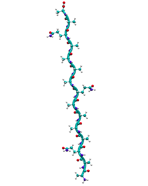
We will perform the simulations in implicit solvent, using the AMBER ff03 force field.
For this tutorial, the following conditions will be explored:
1) 298 K, 1 bar, 0 M
2) 228 K (approach 2 in [6]), 1 bar, 0 M
3) 348 K (approach 2 in [6]), 1 bar, 0 M
4) 298 K, 1 bar, 10 M urea
5) 298 K, 3 kbar, 0 M
Each simulation will be performed for 5 ns.
For the exercises, we will need PLUMED and AMBER. For this purpose, you should first proceed to their installation using the provided conda packages:
#install the PLUMED environment
conda create --name plumed-masterclass-2022
conda activate plumed-masterclass-2022
conda install -c conda-forge plumed py-plumed numpy pandas matplotlib notebook mdtraj mdanalysis git


#install the AMBER environment
conda create --name plumed-masterclass-2022-amber
conda activate plumed-masterclass-2022-amber
conda install -c conda-forge ambertools


#stack the two environments together
conda activate plumed-masterclass-2022
conda activate --stack plumed-masterclass-2022-amber
export PLUMED_KERNEL=/your_path_here/plumed-masterclass-2022/lib/libplumedKernel.so
Then, you should download the folder with the input files for the exercises using the following command:
git clone https://github.com/andrea-arsiccio/masterclass-22-13
In order to perform exercise 1, cd to the folder SASA_module/01_298K. There you will find a number of files:
-aaqaa.prmtop: a topology file of the protein, described according to the AMBER ff03 force field.
-AAQAA_298.in: an input file for running the simulation through AMBER. I will go more in detail over this file in the following.
-aaqaa_min.ncrst/aaqaa_min.pdb: configuration files for the (unfolded) protein, which we will use as starting point for our simulations.
-histograms.py/picture_rg_alpha.gnu/script_rg_alpha.bash: files that we will use for the analyses and postprocessing of our trajectories.
-plumed.dat: PLUMED input file. I will go more in detail over this in the following.
The AAQAA_298.in file is an input AMBER file for carrying out our implicit solvent simulation, and it has the following aspect:
MD Generalise Born, no cut off
 &cntrl
  imin = 0,
  igb = 5, gbsa = 1, extdiel = 78.4, ntpr = 1000, ntwx = 1000, ntwr = 1000,
  ntt = 3, gamma_ln = 1.0, ig = -1, nscm = 500,
  tempi = 298.0, temp0 = 298.0,
  nstlim = 2500000, dt = 0.002, ntc = 2, ntf = 2,
  cut = 9999.0, plumed = 1, plumedfile = 'plumed.dat'
 /
where the different commands have the following meaning:
imin = 0: we are running an MD simulation without performing energy minimization
igb = 5: we are using the model described in https://doi.org/10.1002/prot.20033 for computing the electrostatic interactions \(G^{el}\)
gbsa = 1: the \(G^{np}\) term is also computed
extdiel = 78.4: the dielectric constant of the solvent
ntpr = 1000: we print energy info every 1000 steps
ntwx = 1000: we print coordinates every 1000 steps
ntwr = 1000: we print the restart file every 1000 steps
ntt = 3: we apply Langevin dynamics
gamma_ln = 1.0: we set the collision frequency for Langevin dynamics
ig = -1: seed for pseudo-random number generator. -1 means that the random seed will be based on the current date and time
nscm = 500: translational/rotational COM motions will be removed every 500 steps
tempi = 298.0: initial temperature
temp0 = 298.0: reference temperature at which the system is to be kept
nstlim = 2500000: we will run the system for 2500000 steps
dt = 0.002: we will apply a 2 fs time step
ntc = 2: we will constrain bonds linking to a hydrogen
ntf = 2: bond interactions involving H-atoms will be omitted in force evaluations
cut = 9999.0: no cut off will be applied for nonbonded interactions
plumed = 1: we will run PLUMED together with AMBER
plumedfile = 'plumed.dat': the PLUMED file to read is called plumed.dat
The PLUMED input file plumed.dat has, instead, the following aspect:
MOLINFO MOLTYPE=protein STRUCTURE=aaqaa_min.pdb

# radius of gyration
rgyr: GYRATION TYPE=RADIUS ATOMS=1-174

# antiparallel beta
ab: ANTIBETARMSD RESIDUES=all LESS_THAN={RATIONAL R_0=0.08 NN=8 MM=12} STRANDS_CUTOFF=1

# parallel beta
pb: PARABETARMSD RESIDUES=all LESS_THAN={RATIONAL R_0=0.08 NN=8 MM=12} STRANDS_CUTOFF=1

# alpha helix
alfa: ALPHARMSD RESIDUES=all LESS_THAN={RATIONAL R_0=0.08 NN=8 MM=12}


PRINT ...
 ARG=rgyr,ab.lessthan,pb.lessthan,alfa.lessthan
 STRIDE=1000
 FILE=COLVAR
... PRINT
We are providing PLUMED with a protein structure (aaqaa_min.pdb) in input using the MOLINFO keyword. We are then computing the radius of gyration, parallel/antiparallel beta-sheet content and alpha-helix content of the protein, and we are printing this info to a file called COLVAR every 1000 integration steps. (AAQAA) \(_3\) should fold as a alpha-helix, but we are monitoring also the parallel/antiparallel beta-sheet content in order to identify potential cases of misfolding.
In this first example, we are simulating (AAQAA) \(_3\) in pure water at 298 K and ambient pressure, so we do not need to add the free energy of transfer term \(G^{tr}(T,P,c)\), and the SASA module is not even called in the PLUMED file. However, for exercises 2-5, you will need to use the SASA module to include the effect of temperature/pressure/urea concentration on protein stability.
To run the simulation, just type the command:
sander -O -i AAQAA_298.in -o aaqaa-MD.out -c aaqaa_min.ncrst -p aaqaa.prmtop -r aaqaa-MD.ncrst -x aaqaa-MD.nc >& logfile
The simulation should take 1-2 hours on a common laptop, so you should not need a cluster for this masterclass.
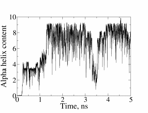
At the end of the simulation, you will have a COLVAR file that lists the evolution of radius of gyration and secondary structure content of the protein as function of time. Try to plot the columns of the COLVAR file versus time. Does the protein fold? If yes, how fast is the process? Do you think the process would be equally fast in explicit solvent?
Here is the evolution of the helical content of (AAQAA) \(_3\) over time during the simulation:
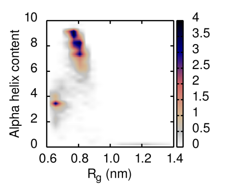
You can also use the script_rg_alpha.bash file provided to have a 2D representation of the conformational space explored by the protein during the simulation. Just type:
chmod +x script_rg_alpha.bash
./script_rg_alpha.bash COLVAR
The script generates a file called normFEL.dat that can be visualized in gnuplot using the picture_rg_alpha.gnu script provided. You should obtain something similar to:
Using the learnings from the theoretical part of this masterclass and exercise 1, you should now be able to autonomously run exercises 2-5. The difference now is that you need to employ free energy of transfer contributions to simulate the solution conditions of exercises 2-5. Exercises 2 and 3 explore extreme (cold and hot) values of temperature. Exercise 4 includes the presence of a potent denaturant (urea), and exercise 5 is performed at a high pressure value.
This means that you will need to use the SASA module, as described in the thoretical summary, to introduce the effect of temperature, pressure and osmolyte concentration within the implicit solvent simulation.
The folder that you downloaded from GitHub contains 5 subfolders, one for each exercise. In each subfolder, every file is ready to use, with the only exception of the plumed.dat file, that you will need to write autonomously using the template employed in exercise 1. Specifically, please monitor for each exercise the radius of gyration and secondary structure content (alpha-helix, parallel and antiparalle beta-sheet) of the protein, and print this information to a file called COLVAR. You will also need to add a SASA_HASEL (hint: use SASA_HASEL instead of SASA_LCPO, as the algorithm by Hasel et al. is faster) and a BIASVALUE section to the plumed.dat file, as discussed in the theoretical section.
You will need to perform the following steps:
-install the software (PLUMED, AMBER)
-clone the GitHub folder with input files: git clone https://github.com/andrea-arsiccio/masterclass-22-13
-write a PLUMED file in each subfolder according to the example of Exercise 1 (hint: use the DeltaG-calculation.py script if needed! The README for the script is available on GitHub, please have a look into it)
-Run the simulations using the command: sander -O -i AAQAA_%%%.in -o aaqaa-MD.out -c aaqaa_min.ncrst -p aaqaa.prmtop -r aaqaa-MD.ncrst -x aaqaa-MD.nc >& logfile
-Analyze the trajectories as already done during exercise 1 (plot the COLVAR columns versus time, and use the script_rg_alpha.bash file to get a representation of the conformational space explored)
You should ask yourself the following questions:
-what would you expect to occur at the protein structure at extreme values of temperature/pressure/urea concentration? Are your expections reflected in the simulation outputs?
-would you observe similar phenomena also in 5-ns-long explicit solvent calculations?
Through this tutorial we have learnt that the SASA module of PLUMED implements two algorithms for the computation of the SASA (the faster algorithm by Hasel et al., and the more accurate LCPO algorithm).
We have found out that the SASA module can be used for introducing the SASA as a collective variable or for monitoring the SASA, but it can furthermore be employed to perform implicit solvent MD simulations.
Implicit solvent simulations with the SASA module are based on the concept of free energy of transfer (where the 'transfer' occurs from pure water at ambient temperature and pressure to an osmolyte solution at any desired value of temperature and pressure).
Implicit solvent simulations have the advantage, compared to their explicit solvent counterpart, to speed up conformational transitions, and allow a faster exploration of conformational space.
NOTE: The Masterclass files with the solutions to the exercises are also avilable on GitHub, but please do the exercises on your own before checking on the results!
 1.8.17