 |
|
|
| |
|
|
The aim of this tutorial is to introduce the users to running a parallel tempering (PT) simulation using PLUMED. We will set up a simple simulation of alanine dipeptide in vacuum, analyze the output, calculate free energies from the simulation, and detect problems. We will also learn how to run a combined PT-metadynamics simulation (PTMetaD) and introduce the users to the Well-Tempered Ensemble (WTE).
In Replica Exchange Methods [81] (REM), sampling is accelerated by modifying the original Hamiltonian of the system. This goal is achieved by simulating N non-interacting replicas of the system, each evolving in parallel according to a different Hamiltonian. At fixed intervals, an exchange of configurations between two replicas is attempted. One popular case of REM is PT, in which replicas are simulated using the same potential energy function, but different temperatures. By accessing high temperatures, replicas are prevented from being trapped in local minima. In PT, exchanges are usually attempted between adjacent temperatures with the following acceptance probability:
\[ p(i \rightarrow j) = min \{ 1,e^{\Delta_{i,j}^{PT}} \}, \]
with
\[ \Delta_{i,j}^{PT} = \left ( \frac{1}{k_B T_i}-\frac{1}{k_B T_j} \right ) \left( U(R_i) - U(R_j) \right ), \]
where \( R_i \) and \( R_j \) are the configurations at temperature \( T_i \) and \( T_j \), respectively. The equation above suggests that the acceptance probability is ultimately determined by the overlap between the energy distributions of two replicas. The efficiency of the algorithm depends on the benefits provided by sampling at high-temperature. Therefore, an efficient diffusion in temperature space is required and configurational sampling is still limited by entropic barriers. Finally, PT scales poorly with system size. In fact, a sufficient overlap between the potential energy distributions of neighboring temperatures is required in order to obtain a significant diffusion in temperature. Therefore, the number of temperatures needed to cover a given temperature range scales as the square root of the number of degrees of freedom, making this approach prohibitively expensive for large systems.
PT can be easily combined with metadynamics [23]. In the resulting PTMetaD algorithm (16), N replicas performed in parallel a metadynamics simulation at different temperatures, using the same set of CVs. The PT acceptance probability must be modified in order to account for the presence of a bias potential:
\[ \Delta_{i,j}^{PTMetaD} = \Delta_{i,j}^{PT} + \frac{1}{k_B T_i} \left [ V_G^{i}(s(R_i),t) - V_G^{i}(s(R_j),t) \right ] + \frac{1}{k_B T_j} \left [ V_G^{j}(s(R_j),t) - V_G^{j}(s(R_i),t) \right ], \]
where \( V_G^{i} \) and \( V_G^{j} \) are the bias potentials acting on the i-th and j-th replicas, respectively.
PTMetaD is particularly effective because it compensates for some of the weaknesses of each method alone. The effect of neglecting a slow degree of freedom in the choice of the metadynamics CVs is alleviated by PT, which allows the system to cross moderately high free-energy barriers on all degrees of freedom. On the other hand, the metadynamics bias potential allows crossing higher barriers on a few selected CVs, in such a way that the sampling efficiency of PTMetaD is greater than that of PT alone.
PTMetaD still suffers from the poor scaling of computational resources with system size. This issue may be circumvented by including the potential energy of the system among the set of well-tempered metadynamics CVs. The well-tempered metadynamics bias leads to the sampling of a well-defined distribution called Well-Tempered Ensemble (WTE) [14]. In this ensemble, the average energy remains close to the canonical value but its fluctuations are enhanced in a tunable way, thus improving sampling.
In the so-called PTMetaD-WTE scheme [38], each replica diffusion in temperature space is enhanced by the increased energy fluctuations at all temperatures.
Once this tutorial is completed students will know how to:
The tarball for this project contains the following directories:
Each directory contains a TOPO subdirectory where topology and configuration files for Gromacs are stored.
Here we use as model systems alanine dipeptide in vacuum and water with AMBER99SB-ILDN all-atom force field.
In this exercise, we will run a PT simulation of alanine dipeptide in vacuum, using only two replicas, one at 300K, the other at 305K. During this simulation, we will monitor the time evolution of the two dihedral angles phi and psi. In order to do that, we need the following PLUMED input file (plumed.dat).
# set up two variables for Phi and Psi dihedral angles
phi: TORSION ATOMS=5,7,9,15
psi: TORSION ATOMS=7,9,15,17

# monitor the two variables
PRINT STRIDE=10 ARG=phi,psi FILE=COLVAR
To submit this simulation with Gromacs, we need the following command line.
mpirun -np 2 gmx_mpi mdrun -s TOPO/topol -plumed -multi 2 -replex 100
This command will execute two MPI processess in parallel, using the topology files topol0.tpr and topol1.tpr stored in the TOPO subdirectory. These two binary files have been created using the usual Gromacs procedure (see Gromacs manual for further details) and setting the temperature of the two simulations at 300K and 305K in the configuration files. An exchange between the configurations of the two simulations will be attempted every 100 steps.
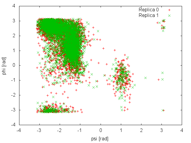
When Gromacs is executed using the -multi option and PLUMED is activated, the output files produced by PLUMED will be renamed and a suffix indicating the replica id will be appended. We will start inspecting the output file COLVAR.0, which reports the time evolution of the CVs at 300K.
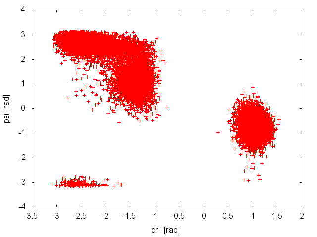
The plot above suggests that during the PT simulation the system is capable to access both the relevant basins in the free-energy surface. This seems to suggest that our simulation is converged. We can use the COLVAR.0 and COLVAR.1 along with the tool sum_hills to estimate the free energy as a function of the CV phi. We will do this a function of simulation time to assess convergence more quantitatively, using the following command line:
plumed sum_hills --histo COLVAR.0 --idw phi --sigma 0.2 --kt 2.5 --outhisto fes_ --stride 1000
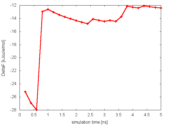
As we did in our previous tutorial, we can now use the script analyze_FES.sh to calculate the free-energy difference between basin A (-3.0<phi<-1.0) and basin B (0.5<phi<1.5), as a function of simulation time.
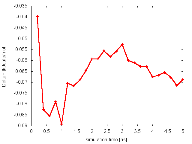
The estimate of the free-energy difference between these two basins seems to be converged. This consideration, along with the observation that the system is exploring all the relevant free-energy basins, might lead us to declare convergence and to state that the difference in free energy between basin A and B is roughly 0 kJoule/mol. Unfortunately, in doing so we would make a big mistake.
In PT simulations we have to be a little bit more careful, and examine the time evolution of each replica diffusing in temperature space, before concluding that our simulation is converged. In order to do that, we need to reconstruct the continuos trajectories of the replicas in temperature from the two files (typically traj0.trr and traj1.trr) which contain the discontinuous trajectories of the system at 300K and 305K. To demux the trajectories, we need to use the following command line:
demux.pl md0.log
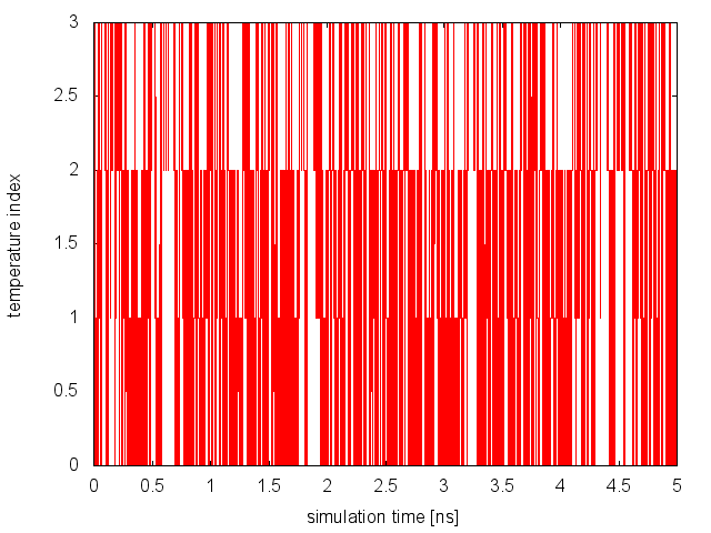
which will create two files, called replica_temp.xvg and replica_index.xvg. We can plot the first file, which reports the temperature index of each configuration at a given time of the simulation. This file is extremely useful, because it allows us monitoring the replicas diffusion in temperature. As we discussed in Summary of theory, in order for the PT algorithm to be effective, we need an efficient diffusion of the replicas in temperature space. In this case, both replicas are rapidly accessing the highest temperature, so there seems not to be any problem on this side.
We can use the second file to reconstruct the continuous trajectories of each replica in temperature:
gmx_mpi trjcat -f traj0.trr traj1.trr -demux replica_index.xvg
and the following PLUMED input file (plumed_demux.dat) to recalculate the value of the CVs on the demuxed trajectories, typically called 0_trajout.xtc and 1_trajout.xtc.
# set up two variables for Phi and Psi dihedral angles
phi: TORSION ATOMS=5,7,9,15
psi: TORSION ATOMS=7,9,15,17

# monitor the two variables
PRINT STRIDE=1 ARG=phi,psi FILE=COLVAR_DEMUX
For the analysis of the demuxed trajectories, we can use the -rerun option of Gromacs, as follows:
# rerun Gromacs on replica 0 trajectory
gmx_mpi mdrun -s TOPO/topol0.tpr -plumed plumed_demux.dat -rerun 0_trajout.xtc
# rename the output
mv COLVAR_DEMUX COLVAR_DEMUX.0
# rerun Gromacs on replica 1 trajectory
gmx_mpi mdrun -s TOPO/topol1.tpr -plumed plumed_demux.dat -rerun 1_trajout.xtc
# rename the output
mv COLVAR_DEMUX COLVAR_DEMUX.1
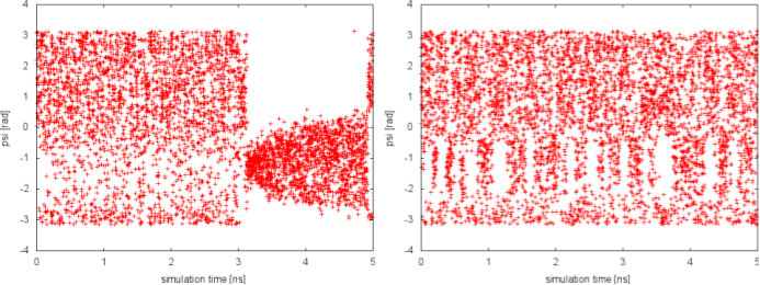
We can now plot the time evolution of the two CVs in the two demuxed trajectories.
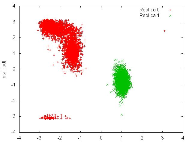
This plot shows clearly that each replica is sampling only one of the two basins of the free-energy landscape, and it is never able to cross the high barrier that separates them. This means that what we considered an exhaustive exploration of the free energy landscape at 300K (Figure belfast-7-pt-fig), was instead caused by an efficient exchange of configurations between replicas that were trapped in different free-energy basins. The results of the present simulation were then influenced by the initial conformations of the two replicas. If we had initialized both of them in the same basin, we would have never observed "transitions" to the other basin at 300K.
To declare convergence of a PT simulation, it is thus mandatory to examine the behavior of the replicas diffusing in temperature and check that these are exploring all the relevant basins. Another good practice is repeating the PT simulation starting from different initial conformations, and check that the results are consistent.
We will now repeat the previous exercise, but with a different setup. The problem with the previous exercise was that replicas were never able to interconvert between the two metastable states of alanine dipeptide in vacuum. The reason was that the highest temperature used (305K) was too low to accelerate barrier crossing in the time scale of the simulation. We will now use 4 replicas at the following temperatures: 300K, 400K, 600K, and 1000K.
We can use the same PLUMED input file described above (plumed.dat), and execute Gromacs using the following command line:
mpirun -np 4 gmx_mpi mdrun -s TOPO/topol -plumed -multi 4 -replex 100
At the end of the simulation, we first monitor the diffusion in temperature space of each replica. We need to create the replica_temp.xvg and replica_index.xvg:
demux.pl md0.log
and plot the content of replica_temp.xvg. Here how it should look for Replica 0:
From this analysis, we can conclude that replicas are diffusing effectively in temperature. Now, we need to monitor the space sampled by each replica while diffusing in temperature space and verify that they are interconverting between the different basins of the free-energy landscape. The demux is carried out as in the previous example:
trjcat_mpi -f traj0.trr traj1.trr traj2.trr traj3.trr -demux replica_index.xvg
and so is the analysis of the demuxed trajectories using the -rerun option of Gromacs and the plumed_demux.dat input file. Here is the space sampled by two of the four replicas:
It is clear that in this case replicas are able to interconvert between the two metastable states, while efficiently diffusing in temperature. We can then calculate the free-energy difference between basin A and B as a function of simulation time at 300K:
and conclude that in this case the PT simulation is converged.
In this exercise we will learn how to combine PT with metadynamics. We will use the setup of the previous exercise, and run a PT simulations with 4 replicas at the following temperatures: 300K, 400K, 600K, and 1000K. Each simulation will perform a well-tempered metadynamics calculation, using the dihedral psi alone as CV and a biasfactor equal to 10 (see Exercise 5. Setup and run a well-tempered metadynamics simulation, part II).
Previously, we prepared a single PLUMED input file to run a PT simulation. This was enough, since in that case the same task was performed at all temperatures. Here instead we need to have a slightly different PLUMED input file for each simulation, since we need to use the keyword TEMP to specify the temperature on the line of the METAD directory. We will thus prepare 4 input files, called plumed.0.dat, plumed.1.dat, plumed.2.dat, and plumed.3.dat, with a different value for the keyword TEMP.
Here how plumed.3.dat should look like:
# set up two variables for Phi and Psi dihedral angles
phi: TORSION ATOMS=5,7,9,15
psi: TORSION ATOMS=7,9,15,17
#
# Activate metadynamics in psi
# depositing a Gaussian every 500 time steps,
# with height equal to 1.2 kJoule/mol,
# and width 0.35 rad.
# Well-tempered metadynamics is activated,
# and the biasfactor is set to 10.0
#
metad: METAD ARG=psi PACE=500 HEIGHT=1.2 SIGMA=0.35 FILE=HILLS BIASFACTOR=10.0 TEMP=1000.0

# monitor the two variables and the metadynamics bias potential
PRINT STRIDE=10 ARG=phi,psi,metad.bias FILE=COLVAR
(see TORSION, METAD, and PRINT).
The PTMetaD simulation is executed in the same way as the PT:
mpirun -np 4 gmx_mpi mdrun -s TOPO/topol -plumed -multi 4 -replex 100
and it will produce one COLVAR and HILLS file per temperature (COLVAR.0, HILLS.0, ...). The analysis of the results requires what we have learned in the previous exercise for the PT case (analysis of the replica diffusion in temperature and demuxing of each replica trajectory), and the post-processing of a well-tempered metadynamics simulation (FES calculation using sum_hills and convergence analysis).
Since in the previous tutorial we performed the same well-tempered metadynamics simulation without the use of PT (see Exercise 5. Setup and run a well-tempered metadynamics simulation, part II), here we can focus on the differences with the PTMetaD simulation. Let's compare the behavior of the biased variable psi in the two simulations:
In well-tempered metadynamics (left panel), the biased variable psi looked stuck early in the simulation (t=3 ns). The reason was the transition of the other hidden degree of freedom phi from one free-energy basin to the other. In the PTMetaD case (right panel), this seems not to happen. To better appreciate the difference, we can plot the time evolution of the hidden degree of freedom phi in the two cases.
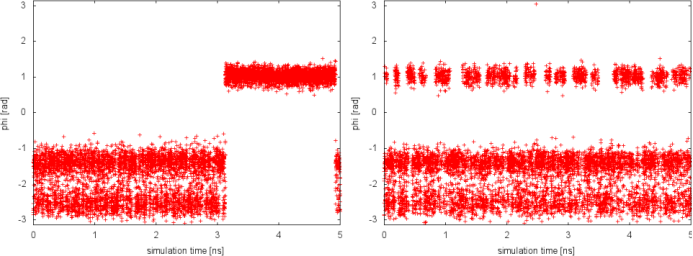
Thanks to the excursions at high temperature, in the PTMetaD simulation the transition of the CV phi between the two basins is accelerate. As a result, the convergence of the reconstructed free energy in psi will be accelerated. This simple exercise demonstrates how PTMetaD can be used to cure a bad choice of metadynamics CVs and the neglecting of slow degrees of freedom.
In this exercise we will learn how to run a PT-WTE and PTMetaD-WTE simulations of alanine dipeptide in water. We will start by running a short PT simulation using 4 replicas in the temperature range between 300K and 400K. We will use a geometric distribution of temperatures, which is valid under the assumption that the specific heat of the system is constant across temperatures. Replicas will thus be simulated at T=300, 330.2, 363.4, and 400K. In this simulation, we will just monitor the two dihedral angles and the total energy of the system, by preparing the following PLUMED input file (plumed_PT.dat):
# set up three variables for Phi and Psi dihedral angles
# and total energy
phi: TORSION ATOMS=5,7,9,15
psi: TORSION ATOMS=7,9,15,17
ene: ENERGY

# monitor the three variables
PRINT STRIDE=10 ARG=phi,psi,ene FILE=COLVAR_PT
(see TORSION, ENERGY, and PRINT).
As usual, the simulation is run for 400ps using the following command:
mpirun -np 4 gmx_mpi mdrun -s TOPO/topol -plumed plumed_PT.dat -multi 4 -replex 100
At the end of the run, we want to analyze the acceptance rate between exchanges. This quantity is reported at the end of the Gromacs output file, typically called md.log, and it can be extracted using the following bash command line:
grep -A2 "Repl average probabilities" md0.log
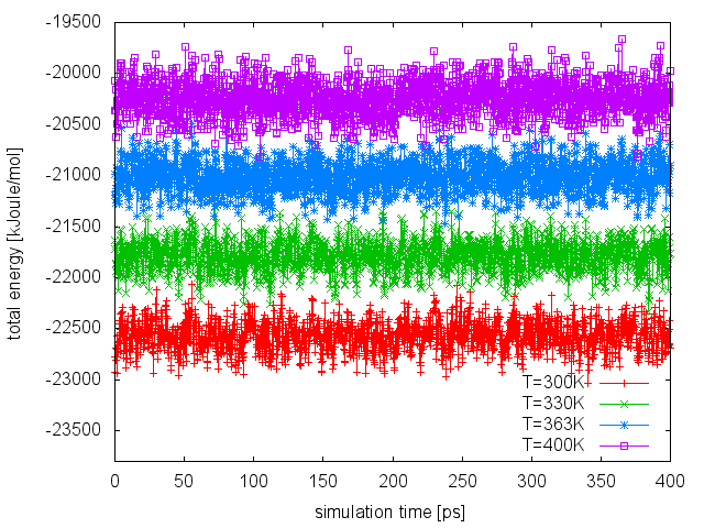
From the line above, we will find out that none of the attempted exchanges has been accepted. The reason is that the current setup (4 replicas to cover the temperature range 300-400K) resulted in a poor overlap of the energy distributions at different temperatures. We can easily realize this by plotting the time series of the total energy in the different replicas:
To improve the overlap of the potential energy distributions at different temperatures, we enlarge the fluctuations of the energy by sampling the Well-Tempered Ensemble (WTE). In order to do that, we need to setup a well-tempered metadynamics simulation using energy as CV. In WTE, fluctuations - the standard deviation of the energy time serie measured above - will be enhanced by a factor equal to the square root of the biasfactor. In this exercise, we will enhance fluctuations of a factor of 4, thus we will set the biasfactor equal to 16. We need to prepare 4 PLUMED input files (plumed_PTWTE.dat.0, plumed_PTWTE.dat.1,...), which will be identical to the following but for the temperature specified in the line of the METAD directive:
# set up three variables for Phi and Psi dihedral angles
# and total energy
phi: TORSION ATOMS=5,7,9,15
psi: TORSION ATOMS=7,9,15,17
ene: ENERGY

# Activate metadynamics in ene
# depositing a Gaussian every 250 time steps,
# with height equal to 1.2 kJoule/mol,
# and width 140 kJoule/mol.
# Well-tempered metadynamics is activated,
# and the biasfactor is set to 16.0
#
wte: METAD ARG=ene PACE=250 HEIGHT=1.2 SIGMA=140.0 FILE=HILLS_PTWTE BIASFACTOR=16.0 TEMP=300.0

# monitor the three variables and the metadynamics bias potential
PRINT STRIDE=10 ARG=phi,psi,ene,wte.bias FILE=COLVAR_PTWTE
(see TORSION, ENERGY, METAD, and PRINT).
Here, we use a Gaussian width larger than usual, and of the order of the fluctuations of the potential energy at 300K, as calculated from the preliminary PT run.
We run the simulation following the usual procedure:
mpirun -np 4 gmx_mpi mdrun -s TOPO/topol -plumed plumed_PTWTE.dat -multi 4 -replex 100
If we analyze the average acceptance probability in this run:
grep -A2 "Repl average probabilities" md0.log
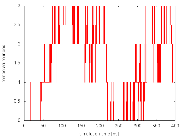
we will notice that now on average 18% of the exchanges are accepted. To monitor the diffusion of each replica in temperature, we can examine the file replica_temp.xvg created by the following command line:
demux.pl md0.log
This analysis assures us that the system is efficiently diffusing in the entire temperature range and no bottlenecks are present.
Finally, as done in the previous run, we can visualize the time serie of the energy CV at all temperatures:
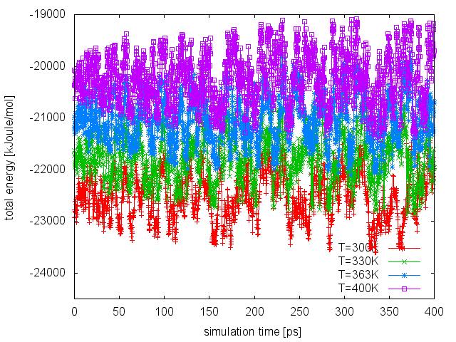
If we compare this plot with the one obtained in the PT run, we can notice that now the enlarged fluctuations caused by the use of WTE lead to a good overlap between energy distributions at different temperatures, thus increasing the exchange acceptance probability. At this point, we can extend our PT-WTE simulation and for example converge the free energy as a function of the dihedral angles phi and psi. Alternatively, we can accelerate sampling of the phi and psi dihedrals by combining PT-WTE with a metadynamics simulation using phi and psi as CVs (PTMetaD-WTE [38]). This can be achieved by preparing 4 PLUMED input files (plumed_PTMetaDWTE.dat.0, plumed_PTMetaDWTE.dat.1,...), which will be identical to the following but for the temperature specified in the two lines containing the METAD directives:
# reload WTE bias
RESTART

# set up three variables for Phi and Psi dihedral angles
# and total energy
phi: TORSION ATOMS=5,7,9,15
psi: TORSION ATOMS=7,9,15,17
ene: ENERGY

# Activate metadynamics in ene
# Old Gaussians will be reloaded to perform
# the second metadynamics run in WTE.
#
wte: METAD ARG=ene PACE=99999999 HEIGHT=1.2 SIGMA=140.0 FILE=HILLS_PTWTE BIASFACTOR=16.0 TEMP=300.0

# Activate metadynamics in phi and psi
# depositing a Gaussian every 500 time steps,
# with height equal to 1.2 kJoule/mol,
# and width 0.35 rad for both CVs.
# Well-tempered metadynamics is activated,
# and the biasfactor is set to 6.0
#
metad: METAD ARG=phi,psi PACE=500 HEIGHT=1.2 SIGMA=0.35,0.35 FILE=HILLS_PTMetaDWTE BIASFACTOR=6.0 TEMP=300.0

# monitor the three variables, the wte and metadynamics bias potentials
PRINT STRIDE=10 ARG=phi,psi,ene,wte.bias,metad.bias FILE=COLVAR_PTMetaDWTE
(see TORSION, ENERGY, METAD, and PRINT).
These scripts activate two metadynamics simulations. One will use the energy as CV and will reload the Gaussians deposited during the preliminary PT-WTE run. No additional Gaussians on this variable will be deposited during the PTMetaD-WTE simulation, due to the large deposition stride. A second metadynamics simulation will be activated on the dihedral angles. Please note the different parameters and biasfactors in the two metadynamics runs.
The simulation is carried out using the usual procedure:
mpirun -np 4 gmx_mpi mdrun -s TOPO/topol -plumed plumed_PTMetaDWTE.dat -multi 4 -replex 100
 1.8.14