 |
|
|
| |
|
|
This document describes the PLUMED tutorial held for the Computational Biology MPhil, University of Cambridge, March 2015. The aim of this tutorial is to learn how to use PLUMED to run well-tempered and bias-exchange simulations and how to run replica-averaged metadynamics to incorporate experimental data into your simulation. Although the presented input files are correct, the users are invited to refer to the literature to understand how the parameters of enhanced sampling methods should be chosen in a real application.
Users are also encouraged to follow the links to the full PLUMED reference documentation and to wander around in the manual to discover the many available features and to do the other, more complete, tutorials. Here we are going to present only a very narrow selection of methods.
Users are expected to write PLUMED input files based on the instructions below.
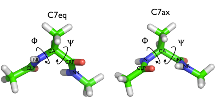
In this tutorial we will play with alanine dipeptide (see Fig. cambridge-1-ala-fig). This rather simple molecule is useful to make many benchmark that are around for data analysis and free energy methods. It is a rather nice example since it presents two metastable states separated by a high (free) energy barrier. Here metastable states are intended as states which have a relatively low free energy compared to adjacent conformation. It is conventional use to show the two states in terms of Ramachandran dihedral angles, which are denoted with \( \Phi \) and \( \Psi \) in Fig. cambridge-1-transition-fig .

The tarball for this project contains all the files needed to run this exercise.
In metadynamics, an external history-dependent bias potential is constructed in the space of a few selected degrees of freedom \(\vec{s}({q}) \), generally called collective variables (CVs) [60]. This potential is built as a sum of Gaussian kernels deposited along the trajectory in the CVs space:
\[ V(\vec{s},t) = \sum_{ k \tau < t} W(k \tau) \exp\left( -\sum_{i=1}^{d} \frac{(s_i-s_i({q}(k \tau)))^2}{2\sigma_i^2} \right). \]
where \( \tau \) is the Gaussian deposition stride, \( \sigma_i \) the width of the Gaussian for the \(i\)th CV, and \( W(k \tau) \) the height of the Gaussian. The effect of the metadynamics bias potential is to push the system away from local minima into visiting new regions of the phase space. Furthermore, in the long time limit, the bias potential converges to minus the free energy as a function of the CVs:
\[ V(\vec{s},t\rightarrow \infty) = -F(\vec{s}) + C. \]
In standard metadynamics, Gaussian kernels of constant height are added for the entire course of a simulation. As a result, the system is eventually pushed to explore high free-energy regions and the estimate of the free energy calculated from the bias potential oscillates around the real value. In well-tempered metadynamics [7], the height of the Gaussian is decreased with simulation time according to:
\[ W (k \tau ) = W_0 \exp \left( -\frac{V(\vec{s}({q}(k \tau)),k \tau)}{k_B\Delta T} \right ), \]
where \( W_0 \) is an initial Gaussian height, \( \Delta T \) an input parameter with the dimension of a temperature, and \( k_B \) the Boltzmann constant. With this rescaling of the Gaussian height, the bias potential smoothly converges in the long time limit, but it does not fully compensate the underlying free energy:
\[ V(\vec{s},t\rightarrow \infty) = -\frac{\Delta T}{T+\Delta T}F(\vec{s}) + C. \]
where \( T \) is the temperature of the system. In the long time limit, the CVs thus sample an ensemble at a temperature \( T+\Delta T \) which is higher than the system temperature \( T \). The parameter \( \Delta T \) can be chosen to regulate the extent of free-energy exploration: \( \Delta T = 0\) corresponds to standard molecular dynamics, \( \Delta T \rightarrow\infty\) to standard metadynamics. In well-tempered metadynamics literature and in PLUMED, you will often encounter the term "bias factor" which is the ratio between the temperature of the CVs ( \( T+\Delta T \)) and the system temperature ( \( T \)):
\[ \gamma = \frac{T+\Delta T}{T}. \]
The bias factor should thus be carefully chosen in order for the relevant free-energy barriers to be crossed efficiently in the time scale of the simulation.
Additional information can be found in the several review papers on metadynamics [59] [8] [93].
In this exercise, we will run a well-tempered metadynamics simulation on alanine dipeptide in vacuum, using as CVs the two backbone dihedral angles phi and psi.
In order to run this simulation we need to prepare the PLUMED input file (plumed.dat) as follows.
# set up two variables for Phi and Psi dihedral angles
phi: TORSION ATOMS=5,7,9,15
psi: TORSION ATOMS=7,9,15,17
#
# Activate metadynamics in phi and psi
# depositing a Gaussian every 500 time steps,
# with height equal to 1.2 kJ/mol,
# and width 0.35 rad for both CVs.
# Well-tempered metadynamics is activated,
# and the biasfactor is set to 6.0
#
metad: METAD ARG=phi,psi PACE=500 HEIGHT=1.2 SIGMA=0.35,0.35 FILE=HILLS BIASFACTOR=6.0

# monitor the two variables and the metadynamics bias potential
PRINT STRIDE=10 ARG=phi,psi,metad.bias FILE=COLVAR
(see TORSION, METAD, and PRINT).
The syntax for the command METAD is simple. The directive is followed by a keyword ARG followed by the labels of the CVs on which the metadynamics potential will act. The keyword PACE determines the stride of Gaussian deposition in number of time steps, while the keyword HEIGHT specifies the height of the Gaussian in kJ/mol. To run well-tempered metadynamics, we need two additional keywords BIASFACTOR and TEMP, which specify how fast the bias potential is decreasing with time and the temperature of the simulation, respectively. For each CVs, one has to specify the width of the Gaussian by using the keyword SIGMA. Gaussian will be written to the file indicated by the keyword FILE.
Once the PLUMED input file is prepared, one has to run Gromacs with the option to activate PLUMED and read the input file:
gmx_mpi mdrun -plumed
During the metadynamics simulation, PLUMED will create two files, named COLVAR and HILLS. The COLVAR file contains all the information specified by the PRINT command, in this case the value of the CVs every 10 steps of simulation, along with the current value of the metadynamics bias potential. The HILLS file contains a list of the Gaussian kernels deposited along the simulation. If we give a look at the header of this file, we can find relevant information about its content. The last column contains the value of the bias factor used, while the last but one the height of the Gaussian, which is scaled during the simulation following the well-tempered recipe.
#! FIELDS time phi psi sigma_phi sigma_psi height biasf
#! SET multivariate false
#! SET min_phi -pi
#! SET max_phi pi
#! SET min_psi -pi
#! SET max_psi pi
      1.0000     -1.3100    0.0525          0.35            0.35      1.4400      6
      2.0000     -1.4054    1.9742          0.35            0.35      1.4400      6
      3.0000     -1.9997    2.5177          0.35            0.35      1.4302      6
      4.0000     -2.2256    2.1929          0.35            0.35      1.3622      6
If we carefully look at the height column, we will notice that in the beginning the value reported is higher than the initial height specified in the input file, which should be 1.2 kJ/mol. In fact, this column reports the height of the Gaussian scaled by the pre-factor that in well-tempered metadynamics relates the bias potential to the free energy. In this way, when we will use sum_hills, the sum of the Gaussian kernels deposited will directly provide the free-energy, without further rescaling needed.
We can plot the time evolution of the CVs along with the height of the Gaussian.
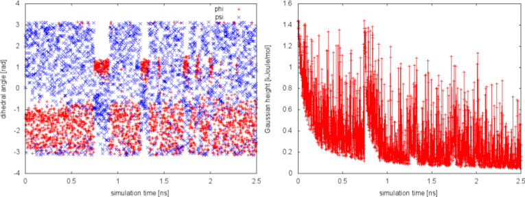
The system is initialized in one of the local minimum where it starts accumulating bias. As the simulation progresses and the bias added grows, the Gaussian height is progressively reduced. After a while (t=0.8 ns), the system is able to escape the local minimum and explore a new region of the phase space. As soon as this happens, the Gaussian height is restored to the initial value and starts to decrease again. In the long time, the Gaussian height becomes smaller and smaller while the system diffuses in the entire CVs space.
One can estimate the free energy as a function of the metadynamics CVs directly from the metadynamics bias potential. In order to do so, the utility sum_hills should be used to sum the Gaussian kernels deposited during the simulation and stored in the HILLS file.
To calculate the two-dimensional free energy as a function of phi and psi, it is sufficient to use the following command line:
plumed sum_hills --hills HILLS
The command above generates a file called fes.dat in which the free-energy surface as function of phi and psi is calculated on a regular grid. One can modify the default name for the free energy file, as well as the boundaries and bin size of the grid, by using the following options of sum_hills :
--outfile - specify the outputfile for sumhills
--min - the lower bounds for the grid
--max - the upper bounds for the grid
--bin - the number of bins for the grid
--spacing - grid spacing, alternative to the number of bins
It is also possible to calculate one-dimensional free energies from the two-dimensional metadynamics simulation. For example, if one is interested in the free energy as a function of the phi dihedral alone, the following command line should be used:
plumed sum_hills --hills HILLS --idw phi --kt 2.5
The result should look like this:
To assess the convergence of a metadynamics simulation, one can calculate the estimate of the free energy as a function of simulation time. At convergence, the reconstructed profiles should be similar. The option –stride should be used to give an estimate of the free energy every N Gaussian kernels deposited, and the option –mintozero can be used to align the profiles by setting the global minimum to zero. If we use the following command line:
plumed sum_hills --hills HILLS --idw phi --kt 2.5 --stride 500 --mintozero
one free energy is calculated every 500 Gaussian kernels deposited, and the global minimum is set to zero in all profiles. Try to visualize the different estimates of the free energy as a function of time.
To assess the convergence of the simulation more quantitatively, we can calculate the free-energy difference between the two local minima in the one-dimensional free energy along phi as a function of simulation time. We can use the bash script analyze_FES.sh to integrate the multiple free-energy profiles in the two basins defined by the following intervals in phi space: basin A, -3<phi<-1, basin B, 0.5<phi<1.5.
./analyze_FES.sh NFES -3.0 -1.0 0.5 1.5 KBT
where NFES is the number of profiles (free-energy estimates at different times of the simulation) generated by the option –stride of sum_hills, and KBT is the temperature in energy units (in this case KBT=2.5).
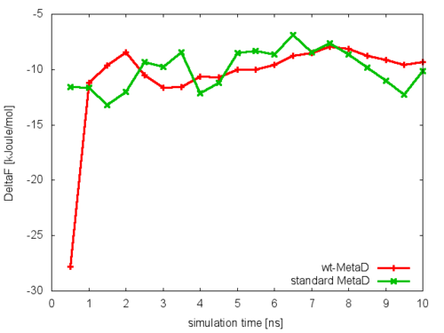
This analysis, along with the observation of the diffusive behavior in the CVs space, suggest that the simulation is converged.
The tarball for this project contains all the files needed to run this exercise.
In well-tempered metadynamics the free-energy landscape of the system is reconstructed by gradually filling the local minima with gaussian hills. The dimensionality of the landscape is equal to the number of CVs which are biased, and typically a number of CVs smaller than four is employed. The reason for this is that qualitatively, if the CVs are not correlated among them, the simulation time required to fill the free-energy landscape grows exponentially with the number of CVs. This limitation can be severe when studying complex transformations or reactions in which more than say three relevant CVs can be identified.
Alternative solutions employ metadynamics together with other enhanced sampling techniques (i.e. Parallel Tempering or more generally Hamiltonian Replica Exchange). In particular in Bias-Exchange metadynamics the problem of sampling a multi-dimensional free-energy surface is recast in that of sampling many one-dimensional free-energies. In this approach a relatively large number N of CVs is chosen to describe the possible transformations of the system (e.g., to study the conformations of a peptide one may consider all the dihedral angles between amino acids). Then, N metadynamics simulations (replicas) are run on the same system at the same temperature, biasing a different CV in each replica. Normally, in these conditions, each bias profile would converge very slowly to the equilibrium free-energy, due to hysteresis.
In order to tackle this problem, in the bias-exchange approach every fixed number of steps (say 10,000) an exchange is attempted between a randomly selected pair of replicas \( a \) and \( b \). The exchanges allow the replicas to gain from the sampling of the other replicas and enable the system to explore the conformational space along a large number of different directions.
The probability to accept the exchange is given by a Metropolis rule:
\[ \min\left( 1, \exp \left[ \beta ( V_G^a(x^a,t)+V_G^b(x^b,t)-V_G^a(x^b,t)-V_G^b(x^a,t) ) \right] \right) \]
where \( x^{a} \) and \( x^{b} \) are the coordinates of replicas \(a \) and \( b \) and \( V_{G}^{a(b)}\left(x,t\right) \) is the metadynamics potential acting on the replica \( a \)( \( b \)). Each trajectory evolves through the high dimensional free energy landscape in the space of the CVs sequentially biased by different metadynamics potentials acting on one CV at each time. The results of the simulation are N one-dimensional projections of the free energy.
In the following example, a bias-exchange simulation is performed on Alanine di-peptide. A typical input file for bias exchange well tempered metadynamics is the following:
plumed-common.dat:

# read a pdb file to get topology info
MOLINFO STRUCTURE=ALAD.pdb

# tell PLUMED to generate random exchange trials
RANDOM_EXCHANGES

# set up four variables for Phi, Psi, Theta, Xi dihedral angles
phi: TORSION ATOMS=@phi-2
psi: TORSION ATOMS=@psi-2
theta: TORSION ATOMS=6,5,7,9
xi: TORSION ATOMS=16,15,17,19

PRINT ARG=phi,psi,theta,xi STRIDE=250 FILE=COLVAR
(see MOLINFO and RANDOM_EXCHANGES).
plumed.dat.0:

INCLUDE FILE=plumed-common.dat
METAD ARG=phi HEIGHT=1.2 SIGMA=0.25 PACE=100 GRID_MIN=-pi GRID_MAX=pi BIASFACTOR=10.0
ENDPLUMED


plumed.dat.1:

INCLUDE FILE=plumed-common.dat
METAD ARG=psi HEIGHT=1.2 SIGMA=0.25 PACE=100 GRID_MIN=-pi GRID_MAX=pi BIASFACTOR=10.0
ENDPLUMED


plumed.dat.2:

INCLUDE FILE=plumed-common.dat
METAD ARG=theta HEIGHT=1.2 SIGMA=0.50 PACE=100 GRID_MIN=-pi GRID_MAX=pi BIASFACTOR=10.0
ENDPLUMED


plumed.dat.3:

INCLUDE FILE=plumed-common.dat
METAD ARG=xi HEIGHT=1.2 SIGMA=0.50 PACE=100 GRID_MIN=-pi GRID_MAX=pi BIASFACTOR=10.0
ENDPLUMED
The, in this case, two replicas start from the same GROMACS topology file replicated twice: topol0.tpr, topol1.tpr, topol2.tpr and topol3.tpr. Finally, GROMACS is launched as a parallel run on 4 cores, with one replica per core, with the command
mpirun -np 4 gmx_mpi mdrun -s topol -plumed plumed -multi 4 -replex 10000 >& log &
where -replex 10000 indicates that every 10000 molecular-dynamics steps exchanges are attempted (as printed in the GROMACS *.log files).
In order to have an idea of how Bias-Exchange Metadynamics works we can compare the sampling of the four replicas along the first two collective variables with respect to a free energy surface obtained by sampling in two dimensions.
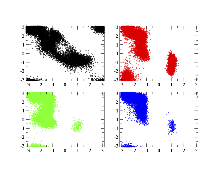
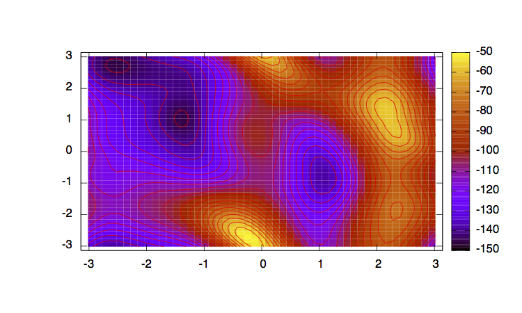
The main features are that all the replicas can sample all the relevant free energy minima even if their collective variable is not meant to sample them, only the replicas with a collective variable meant to pass a barrier can sample that transition, so high energy regions are sampled only locally. This can seem a weakness in the case of alanine dipeptide but is the real strength of bias exchange metadynamics, indeed by not knowing anything of a system it is possible to choose as many collective variables as possible and even if most of them are not particularly useful a posteriori, they all gain from the good ones and nothing is lost.
As for the former case, one can estimate the free energy as a function of the metadynamics CVs directly from the metadynamics bias potential. This approach can only be used to recover one-dimensional free-energy profiles:
plumed sum_hills --hills HILLS.0 --mintozero
The command above generates a file called fes.dat in which the free-energy surface as function of phi is calculated on a regular grid.
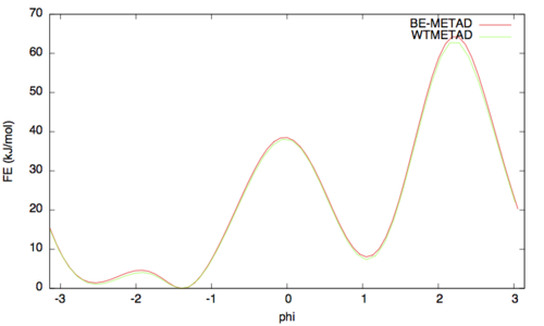
It is also possible to calculate one-dimensional free energies from the two-dimensional metadynamics simulation. For example, if one is interested in the free energy as a function of the phi dihedral alone, the following command line should be used:
The result should look like this (compared with the one obtained before):
As above we can assess the convergence of a metadynamics simulation by calculating the estimate of the free energy as a function of simulation time. At convergence, the reconstructed profiles should be similar. The option –stride should be used to give an estimate of the free energy every N Gaussian kernels deposited, and the option –mintozero can be used to align the profiles by setting the global minimum to zero. If we use the following command line:
plumed sum_hills --hills HILLS.0 --stride 500 --mintozero
Try to visualize the different estimates of the free energy as a function of time.
To assess the convergence of the simulation more quantitatively, we can calculate the free-energy difference between the two local minima in the one-dimensional free energy along phi as a function of simulation time. We can use the bash script analyze_FES.sh to integrate the multiple free-energy profiles in the two basins defined by the following intervals in phi space: basin A, -3<phi<-1, basin B, 0.5<phi<1.5.
./analyze_FES.sh NFES -3.0 -1.0 0.5 1.5 KBT
where NFES is the number of profiles (free-energy estimates at different times of the simulation) generated by the option –stride of sum_hills, and KBT is the temperature in energy units (in this case KBT=2.5).
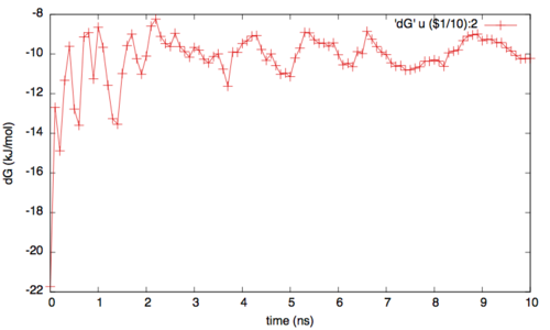
In addition to check for the convergence of the one dimesional profiles, it is important to verify the rate of exchange among the replicas. In fact if the rate is too low or if it is not enough homegenues then the replicas can still suffer from histeris problems (ie with one replica trapped somewhere in the conformational space). Generally speaking a good probability of exchange is between 10 and 30%.
It is possible to check the exchange statistics and the detailed diffusion of the replicas among the different biases using a script provided:
./demux_m.pl md0.log
which will create two files, called replica_temp.xvg and replica_index.xvg. We can plot the first file, which reports the bias index of each configuration at a given time of the simulation. This file is extremely useful, because it allows us monitoring the replicas diffusion in bias.
The tarball for this project contains all the files needed to run this exercise.
Equilibrium experimental data are the result of a measure over an ensemble of structures and over time. In principle a "perfect" molecular dynamics simulations, that is a simulations with a perfect force-field and a perfect sampling can predict the outcome of an experiment in a quantitative way. Actually in most of the cases obtaining a qualitative agreement is already a fortunate outcome. In order to increase the accuracy of a force field in a system dependent manner it is possible to add to the force-field an additional term based on the agreement with a set of experimental data. This agreement is not enforced as a simple restraint because this would mean to ask the system to be always in agreement with all the experimental data at the same time, instead the restraint is applied over an AVERAGED COLLECTIVE VARIABLE where the average is performed over multiple identical simulations (replicas). In this way there is not a single replica that must be in agreement with the experimental data but they should be in agreement on average. It has been shown that this approach is equivalent to solve the problem of finding a modified version of the force field that reproduces the provided set of experimental data without any additional assumption on the data themselves [34] [32] [26] [19] .
In this exercise we will model the equilibrium ensemble of Chignolin by combining an implicit solvent force-field (Amber99sb) with synthetic experimental data derived from an experimentally determined ensemble of structures.
The experimental data are the following distances among CA carbons that have been averaged over the whole ensemble.
#RES RES DISTANCE(nm)
 1   3   0.656214
 1   4   0.963703
 1   5   1.197160
 1   6   1.219970
 1   7   1.206760
 1   8   1.060110
 1   9   0.858911
 1  10   0.872988
 2   4   0.656913
 2   5   0.931405
 2   6   0.953046
 2   7   0.901493
 2   8   0.809623
 2   9   0.716444
 2  10   0.882070
 3   5   0.588322
 3   6   0.660023
 3   7   0.704165
 3   8   0.720063
 3   9   0.799961
 3  10   0.981838
 4   6   0.550374
 4   7   0.572299
 4   8   0.764540
 4   9   0.939752
 4  10   1.186040
 5   7   0.613088
 5   8   0.847734
 5   9   1.084080
 5  10   1.296630
 6   8   0.591571
 6   9   0.888388
 6  10   1.102920
 7   9   0.701717
 7  10   0.987368
 8  10   0.654310
Here we will give partial information on how to setup the simulations. Users should refer to the manual and the literature cited on how to complete the information provided and thus successfully perform the exercise.
Step 1: Add the collective variables that describe the distances averaged over the ensemble to the template input files provided.
For each of the above experimental data one should define:
#this is the distance between CA atoms 5 and 33 belonging to residues 1 and 3, respectively.
d1: DISTANCE ATOMS=5,33
# this is the averaging of the distance among the replicas
ed1: ENSEMBLE ARG=d1
# this is the restraint applied on the averaged distance to match the experimental one
RESTRAINT ARG=ed1.d1 KAPPA=100000 AT=0.656214
(see DISTANCE, ENSEMBLE, and RESTRAINT).
Step 2: Setup the Bias-Exchange simulations
We will run Bias-Exchange simulations using four CVs, two of them have already been chosen (see plumed-common.dat) while the others should be selected by you. Additionally Metadynamics parameters METAD for the two selected collective variables should be added in the plumed.dat.0 and plumed.dat.1 files. In particular while the PACE, HEIGHT and BIASFACTOR can be kept the same of those defined for the selected CVs, the SIGMA should be half of the fluctuations of the chosen CV in an unbiased run (>1 ns).
Step 3: Run
The simulation should be run until convergence of the four one dimensional free energies, this will typically take more than 200 ns per replica.
Step 4: Analysis
The user should check the diffusion of the replicas among the biases (see above) and send the converged free energy profiles.
Step 5: Only for the brave!
The same simulation without experimental restraints could be performed in such a way to compare the free energy profiles obtained with and without the inclusion of experimental data.
 1.8.14