 |
|
|
| |
|
|
The aim of this tutorial is to show how to use PLUMED to run simulations with multiple replicas and how to analyze them. In particular, we will focus on cases where the replicas feel different biasing potentials.
Once this tutorial is completed students will be able to:
The TARBALL for this project contains the following files:
topol0.tpr, topol1.tpr, topol2.tpr, and topol3.tpr, gromacs input files for analine dipeptide. Notice that two of them (0 and 2) are initialized in one free-energy well and two of them (1 and 3) in the other free-energy well.wham.py script to perform WHAM. Notice that this required python 3 (does not work with python 2).This tutorial has been tested on a pre-release version of version 2.4. In particular, it takes advantage of a special syntax for setting up multi-replica simulations that is only available since version 2.4. Exercise could be done also with version 2.3 but using a different syntax with respect to the one suggested.
Also notice that in the .solutions directory of the tarball you will find correct input files. Please only look at these files after you have tried to solve the problems yourself.
So far we always used PLUMED to run one simulation at a time. However, PLUMED can also be used in multi-replica algorithms. When coupled with GROMACS (at least) it is also possible to run replica exchange simulations, where coordinates are swapped from time to time. In this case, PLUMED is going to take into account the different bias potentials applied to different replicas so as to compute correctly the acceptance.
Similarly to what we did before, we will first use the driver to understand how to prepare multi-replica input files. However, the very same holds when you run multi-replica MD simulations with MD codes that support them. For instance, in GROMACS that would be using the -multi option of mdrun.
Notice that this tutorial was tested using a pre-release version of PLUMED 2.4. In particular, we will use a special syntax for multi-replica input that is only available starting with PLUMED 2.4.
Imagine that you are in a directory with these files
traj.0.xtc
traj.1.xtc
traj.2.xtc
plumed.dat
That is: three trajectories and a PLUMED input files. Let's say that the content of plumed.dat is
d: DISTANCE ATOMS=1,2
PRINT ARG=d FILE=COLVAR
You can use the following command to process the three trajectories simultaneously:
mpirun -np 3 plumed driver --multi 3 --plumed plumed.dat --mf_xtc traj.xtc
This command will produce three COLVAR files, namely COLVAR.0, COLVAR.1, and COLVAR.2.
How does this work?
You are here running three replicas of the plumed executable. When PLUMED opens a file for writing it adds a a suffix corresponding to the replica number. This is done for all the possible files written by PLUMED and allows you to distinguish the output of different replicas redirecting it to different files.
plumed.dat file. If by mistake you include an additional plumed.0.dat file in the same directory, PLUMED will use that file for replica 0 (and plumed.dat for replicas 1 and 2). To be precise, this is true for all the files read by PLUMED, with the exception of PDB files where the suffix is never added.The last comment implies that if you need to process your trajectories with different input files you might do it creating files named plumed.0.dat, plumed.1.dat, and plumed.2.dat. This is correct, and this was the only way to do multi-replica simulations with different input files up to PLUMED 2.3. However, in the following we will see how to obtain the same effect with a new special command that has been introduced in PLUMED 2.4.
In many cases, we need to run multiple replicas with almost identical PLUMED files. These files might be prepared with cut-and-paste, which is very error prone, or could be set up with some smart bash or python script. Additionally, one can take advantage of the INCLUDE keyword so as to have a shared input file with common definitions and specific input files with replica-dependent keywords. However, as of PLUMED 2.4, we introduced a simpler manner to manipulate multiple replica inputs with tiny differences. Look at the following example:
#SETTINGS NREPLICAS=3
# Compute a distance
d: DISTANCE ATOMS=1,2

# Apply a restraint.
RESTRAINT ARG=d AT=@replicas:1.0,1.1,1.2 KAPPA=1.0
# On replica 0, this means:
#   RESTRAINT ARG=d AT=1.0 KAPPA=1.0
# On replica 1, this means:
#   RESTRAINT ARG=d AT=1.1 KAPPA=1.0
# On replica 2, this means:
#   RESTRAINT ARG=d AT=1.2 KAPPA=1.0
If you prepare a single plumed.dat file like this one and feeds it to PLUMED while using 3 replicas, the 3 replicas will see the very same input except for the AT keyword, that sets the position of the restraint. Replica 0 will see a restraint centered at 1.0, replica 1 centered at 1.1, and replica 2 centered at 1.2.
The @replicas: keyword is not special for RESTRAINT or for the AT keyword. Any keyword in PLUMED can accept that syntax. For instance, the following single input file can be used to setup a bias exchange metadynamics [80] simulations:
#SETTINGS NREPLICAS=2
# Compute distance between atoms 1 and 2
d: DISTANCE ATOMS=1,2

# Compute a torsional angle
t: TORSION ATOMS=30,31,32,33

# Metadynamics.
METAD ...
  ARG=@replicas:d,t
  HEIGHT=1.0
  PACE=100
  SIGMA=@replicas:0.1,0.3
  GRID_MIN=@replicas:0.0,-pi
  GRID_MAX=@replicas:2.0,pi
...
# On replica 0, this means:
#  METAD ARG=d HEIGHT=1.0 PACE=100 SIGMA=0.1 GRID_MIN=0.0 GRID_MAX=2.0
# On replica 1, this means:
#  METAD ARG=t HEIGHT=1.0 PACE=100 SIGMA=0.3 GRID_MIN=-pi GRID_MAX=pi
This would be a typical setup for a bias exchange simulation. Notice that even though variables d and t are both read in both replicas, d is only computed on replica 0 (and t is only computed on replica 1). This is because variables that are defined but not used are never actually calculated by PLUMED.
If the value that should be provided for each replica is a vector, you should use curly braces as delimiters. For instance, if the restraint acts on two variables, you can use the following input:
#SETTINGS NREPLICAS=3
# Compute distance between atoms 1 and 2
d: DISTANCE ATOMS=10,20

# Compute a torsional angle
t: TORSION ATOMS=30,31,32,33

# Apply a restraint:
RESTRAINT ...
  ARG=d,t
  AT=@replicas:{{1.0,2.0} {3.0,4.0} {5.0,6.0}}
  KAPPA=1.0,3.0
...
# On replica 0 this means:
#  RESTRAINT ARG=d AT=1.0,2.0 KAPPA=1.0,3.0
# On replica 1 this means:
#  RESTRAINT ARG=d AT=3.0,4.0 KAPPA=1.0,3.0
# On replica 2 this means:
#  RESTRAINT ARG=d AT=5.0,6.0 KAPPA=1.0,3.0
Notice the double curly braces. The outer ones are used by PLUMED to know there the argument of the AT keyword ends, whereas the inner ones are used to group the values corresponding to each replica. Also notice that the last example can be split in multiple lines exploiting the fact that within multi-line statements (enclosed by pairs of ...) newlines are replaced with simple spaces:
#SETTINGS NREPLICAS=3
d: DISTANCE ATOMS=10,20
t: TORSION ATOMS=30,31,32,33
RESTRAINT ...
  ARG=d,t
# indentation is not required (this is not python!)
# but makes the input easier to read
  AT=@replicas:{
    {1.0,2.0}
    {3.0,4.0}
    {5.0,6.0}
  }
  KAPPA=1.0,1.0
...
In short, whenever there are keywords that should vary across replicas, you should set them using the @replicas: keyword. As mentioned above, you can always use the old syntax with separate input file, and this is recommended when the number of keywords that are different is large.
Write a plumed file that allows you to run a multi-replica simulation of alanine dipeptide where the following four replicas are simulated:
With PLUMED 2.3 you should use four plumed.dat files (named plumed.0.dat, plumed.1.dat, etc). In this case, the first two replicas feel no potential, so you could just use empty files. For the third and fourth replica you could recycle the files from Trieste tutorial: Metadynamics simulations with PLUMED.
However, we recommend you to take the occasion to make practice with the special replica syntax of PLUMED 2.4. Use the following input file as a starting point
# load the pdb to better select torsions later
MOLINFO __FILL__
# Compute the backbone dihedral angle phi, defined by atoms C-N-CA-C
phi: TORSION ATOMS=__FILL__
# Compute the backbone dihedral angle psi, defined by atoms N-CA-C-N
psi: TORSION ATOMS=__FILL__

metad: METAD ...
# Activate well-tempered metadynamics
# Deposit a Gaussian every 500 time steps, with initial height equal
# to 1.2 kJoule/mol, biasfactor equal to 10.0
# Remember: replica 0 and 1: no bias
# replica 2, bias on phi
# replica 3, bias on psi
  ARG=__FILL__
  HEIGHT=__FILL__ # make sure that replicas 0 and 1 feel no potential!
  PACE=500
  BIASFACTOR=10.0
  SIGMA=0.35
# Gaussians will be written to file and also stored on grid
  FILE=HILLS GRID_MIN=-pi GRID_MAX=pi
...

# Print both collective variables and the value of the bias potential on COLVAR file
PRINT ARG=__FILL__ FILE=COLVAR STRIDE=10
Now check the resources provided with this tutorial. There are 4 tpr files available (topol0.tpr, topol1.tpr, topol2.tpr, and topol3.tpr). You can run a replica exchange simulation with gromacs using the following command
> mpirun -np 4 gmx_mpi mdrun -plumed plumed.dat -nsteps 1000000 -replex 120 -multi 4
Notice that coordinates swaps will be attempted between different replicas every 120 steps. When computing the acceptance, gromacs will take into account that different replicas might be subject to different bias potential. In this example, replicas 0 and 1 are actually subject to the same potential, so all the exchanges will be accepted. You can verify this using the command
> grep "Repl ex" md0.log
It is interesting to see what happens at different stages of the simulation. At the beginning of the trajectory you should see something like this
> grep "Repl ex" md0.log | head
Repl ex  0 x  1    2 x  3
Repl ex  0    1 x  2    3
Repl ex  0 x  1    2 x  3
Repl ex  0    1 x  2    3
Repl ex  0 x  1    2 x  3
Repl ex  0    1    2    3
Repl ex  0 x  1    2 x  3
Repl ex  0    1 x  2    3
Repl ex  0 x  1    2 x  3
Repl ex  0    1 x  2    3
Notice that all the exchanges between replicas 0 and 1 are accepted and also almost all the exchanges between replicas 1, 2, and 3. At a later stage you will more likely find something like this
> grep "Repl ex" md0.log | tail
Repl ex  0    1 x  2    3
Repl ex  0 x  1    2    3
Repl ex  0    1 x  2    3
Repl ex  0 x  1    2    3
Repl ex  0    1 x  2    3
Repl ex  0 x  1    2 x  3
Repl ex  0    1 x  2    3
Repl ex  0 x  1    2 x  3
Repl ex  0    1    2    3
Repl ex  0 x  1    2    3
Notice that all the exchanges between replicas 0 and 1 are still accepted. This is because the potential energy felt by replicas 0 and 1 are identical. However, exchanges between replicas 1, 2, and 3 are sometime rejected.
In the following we will analyze the result of the simulation above. To this aim we will have to use the WHAM method. The WHAM procedure described here is binless and allows one to reweight arbitrary bias potentials without the need to discretize collective variables. As a first step it is necessary to create a concatenated trajectory that includes all the conformations that you produced during your simulations.
> gmx_mpi trjcat -f traj_comp*.xtc -cat -o fulltraj.xtc
Notice that a new trajectory file fulltraj.xtc will be in your working directory now, approximately four times bigger than the individual files traj_comp*.xtc.
Now we will process that directory computing the bias potentials associated with the replicas that we simulated. Similarly to what we did in Trieste tutorial: Metadynamics simulations with PLUMED, we will assume that reweighting is done with final bias potential [22]. Notice that also here it would be possible to use [95] instead.
# this will be file plumed_reweight.dat
# include here exactly the same file you used to run the simulation
# however, you should make some change to METAD:
# - replace PACE with a huge number
# - add TEMP=300 to set the temperature of the simulation
# (normally this is inherited from the MD code, but driver has no idea about it)
# - add RESTART=YES to trigger restart
__FILL__
__FILL__
__FILL__
__FILL__
# you should also change the PRINT command so as not to overwrite
# the files you wrote before.
# here omit STRIDE, so that you will print
# for all the frames in your concatenated trajectory
PRINT ARG=phi,psi FILE=COLVAR_CONCAT

# Then write the bias potential (as we did for reweighting)
# As a good practice, remember that there might be multiple bias
# potential applied (e.g. METAD and a RESTRAINT).
# to be sure that you include all of them, just combine them:
bias: COMBINE ARG=*.bias PERIODIC=NO
# here omit STRIDE, so that you will print the bias
# for all the frames in your concatenated trajectory
PRINT FILE=COLVAR_WHAM ARG=bias
Then analyze the concatenated trajectory with this command
> mpirun -np 4 plumed driver --mf_xtc fulltraj.xtc --plumed plumed_reweight.dat --multi 4
Notice that since fulltraj.xtc the four concurrent copies of PLUMED will all analyze the same trajectory, which is what we want to do now. The result will be a number of COLVAR_WHAM files, one per replica, with a number of lines corresponding to the whole concatenated trajectory.
# put the bias columns in a single file ALLBIAS
> paste COLVAR_WHAM.* | grep -v \# | awk '{for(i=1;i<=NF/2;i++) printf($(i*2)"  ");printf("\n");}' > ALLBIAS
Have a look at ALLBIAS. It should look more or less like this
0.000000  0.000000  75.453800  68.172206
0.000000  0.000000  74.973726  68.143015
0.000000  0.000000  66.948910  56.295899
0.000000  0.000000  70.383309  60.164381
0.000000  0.000000  65.595489  61.754951
0.000000  0.000000  67.689166  60.869430
The first two columns correspond to the bias felt in replicas 0 and 1, that are unbiased, and thus should be zero. In the other replicas on the other hand we will have large potentials accumulated by metadynamics. The actual numbers might very depending on the length of your simulation.
Now you can use the provided python script to analyze the ALLBIAS file. SCRIPTS/wham.py should be provided three arguments: name of the file with bias potentials, number of replicas (that is the number of columns) and value of k \(_B\)T (2.5 in kj/mol).
# use the python script to compute weights
> python3 SCRIPTS/wham.py ALLBIAS 4 2.5
This will generate a file named weights.dat that contains the weights for each of the frame. The initial values reported in the file should be similar to these ones:
> head weights.dat
 3.688530731178e-05
3.899877363004e-05
7.861996862568e-07
3.663355487180e-06
1.647251040152e-06
2.689614526429e-06
3.254124396415e-06
1.511057459698e-05
2.342149322226e-05
5.032261109943e-06
Weights are very small since we have a long trajectory with many frames. You can check that they are normalized using the command ‘awk ’{a+=$1}END{print a}' weights.dat`.
Now have a look at the weights. Remember that we are concatenating trajectories.
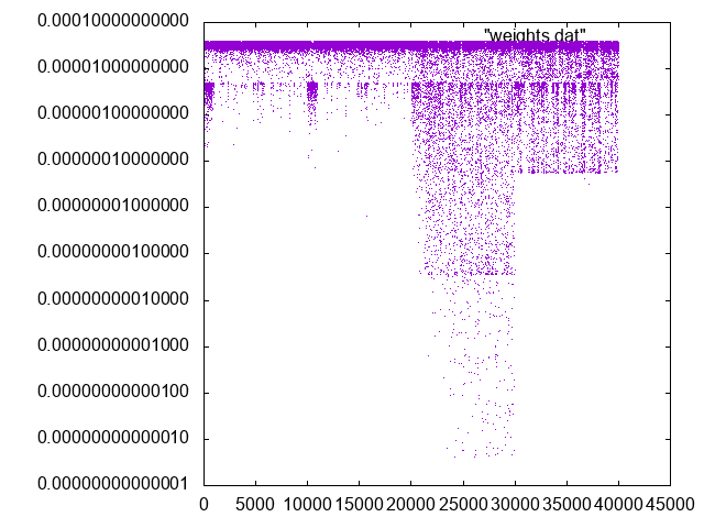
Can you understand why weights in the first half are systematically different from weights in the second half? The first part correspond to the unbiased trajectories. All the snapshots sampled here are reasonably correct. However, in the second part we have heavily biased snapshots, which also sample transition states. Those points are assigned a low weight by WHAM so that they would be discarded in the calculation of any unbiased average.
Now we have the weight for each frame. We would like to compute the relative stability of the two free-energy wells that correspond roughly to positive and negative \(\phi\).
> paste <(grep -v \# COLVAR_CONCAT.0) weights.dat | awk '{if($2>0)wb+=$NF; else wa+=$NF}END{print wa,wb}'
This will tell you the unbiased population of the two minima. You should expect values close to these ones
0.968885 0.0311148
that tells you that the first minimum has a population of roughly 97%.
Repeat the exercise above (that is: running replica exchange MD simulation and analyze the result) but using only three replicas:
Create a file plumed3.dat aimed at this. If you are not able you can find a working one in the solutions directory. Then use the following commands similarly to before:
> mpirun -np 3 gmx_mpi mdrun -plumed plumed3.dat -nsteps 1000000 -replex 120 -multi 3
> gmx_mpi trjcat -f traj_comp{0,1,2}.xtc -cat -o fulltraj.xtc
> mpirun -np 3 plumed driver --mf_xtc fulltraj.xtc --plumed plumed3_reweight.dat --multi 3
> paste COLVAR_WHAM.{0,1,2} | grep -v \# | awk '{for(i=1;i<=NF/2;i++) printf($(i*2)"  ");printf("\n");}' > ALLBIAS
> python3 SCRIPTS/wham.py ALLBIAS 3 2.5
Compute as before the relative population of the two minima.
> paste <(grep -v \# COLVAR_CONCAT.0) weights.dat | awk '{if($2>0)wb+=$NF; else wa+=$NF}END{print wa,wb}'
Which is the result? What can you learn from this example?
If you did things correctly, here you should find a population close to 2/3 for the first minimum and 1/3 for the second one. Notice that this population just reflects the way we initialized the simulations (2 of them in one minimum and 1 in the other minimum) and does not take into account which is the relative stability of the two minima according to the real potential energy function. In other words, we are just obtaining the relative population that we used to initialize the simulation.
Also plot the colvar files and look at them with attention. An excerpt is shown below.
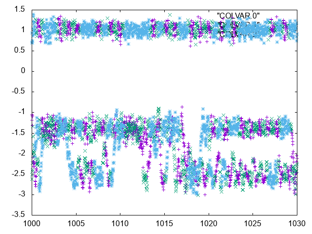
always due to accepted exchanges between replicas."
How many transitions between the two free-energy wells can you observe? Remember that replica exchange involves coordinate swaps that do not correspond to the real system dynamics. It is very useful to look at "demuxed" trajectories.
Use the following commands
> demux.pl md0.log
This will produce two files: replica_index.xvg and replica_temp.xvg. The former allows to convert your trajectories to continuous ones with the following commands
> demux.pl md0.log
> gmx_mpi  trjcat -f traj_comp?.xtc -demux replica_index.xvg
You will now find new trajectories 0_trajout.xtc, 1_trajout.xtc, 2_trajout.xtc, and 3_trajout.xtc. These files can be in turn analyzed with plumed driver. Try to recompute collective variables on the trajectories obtained in Exercise 1: Running multi-replica simulations and with those obtained in Exercise 3: What if a variable is missing?.
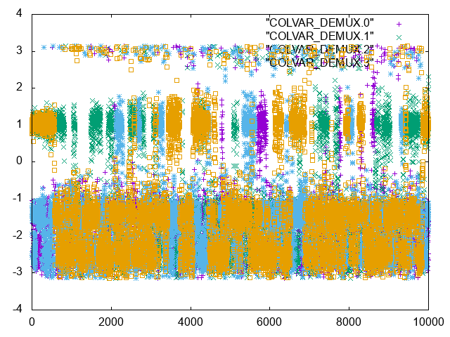
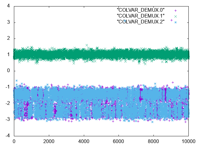
As you can see, the trajectories from Exercise 1: Running multi-replica simulations show a number of transitions. On the other hand, the trajectories from Exercise 3: What if a variable is missing? are stuck.
As a general rule, notice that there is no way to estimate correctly the relative population of two metastable states if there is not a continuous "demuxed" trajectory joining them, possibly exhibiting multiple transitions.
In summary, in this tutorial you should have learned how to use PLUMED to:
Notice that the setup used is similar to the ones typically used in bias exchange simulations but can be easily adapted to any case where multiple replicas should be combined that feel different bias potentials. Moreover, the problematic example discussed shows that one should be careful and check if real transitions are observed during a replica exchange simulation.
 1.8.14