 |
|
|
| |
|
|
The aim of this tutorial is to introduce the users to running a metadynamics simulation with PLUMED. We will set up a simple simulation of alanine dipeptide in vacuum, analyze the output, and estimate free energies from the simulation. We will also learn how to run a well-tempered metadynamics simulation and detect issues related to a bad choice of collective variables.
In metadynamics, an external history-dependent bias potential is constructed in the space of a few selected degrees of freedom \(\vec{s}({q}) \), generally called collective variables (CVs) [64]. This potential is built as a sum of Gaussian kernels deposited along the trajectory in the CVs space:
\[ V(\vec{s},t) = \sum_{ k \tau < t} W(k \tau) \exp\left( -\sum_{i=1}^{d} \frac{(s_i-s_i({q}(k \tau)))^2}{2\sigma_i^2} \right). \]
where \( \tau \) is the Gaussian deposition stride, \( \sigma_i \) the width of the Gaussian for the \(i\)th CV, and \( W(k \tau) \) the height of the Gaussian. The effect of the metadynamics bias potential is to push the system away from any local minimum and into visiting new regions of the phase space. Furthermore, in the long time limit, the bias potential converges to minus the free energy as a function of the CVs:
\[ V(\vec{s},t\rightarrow \infty) = -F(\vec{s}) + C. \]
In standard metadynamics, Gaussian kernels of constant height are added for the entire course of a simulation. As a result, the system is eventually pushed to explore high free-energy regions and the estimate of the free energy calculated from the bias potential oscillates around the real value. In well-tempered metadynamics [8], the height of the Gaussian is decreased with simulation time according to:
\[ W (k \tau ) = W_0 \exp \left( -\frac{V(\vec{s}({q}(k \tau)),k \tau)}{k_B\Delta T} \right ), \]
where \( W_0 \) is an initial Gaussian height, \( \Delta T \) an input parameter with the dimension of a temperature, and \( k_B \) the Boltzmann constant. With this rescaling of the Gaussian height, the bias potential smoothly converges in the long time limit, but it does not fully compensate the underlying free energy:
\[ V(\vec{s},t\rightarrow \infty) = -\frac{\Delta T}{T+\Delta T}F(\vec{s}) + C. \]
where \( T \) is the temperature of the system. In the long time limit, the CVs thus sample an ensemble at a temperature \( T+\Delta T \) which is higher than the system temperature \( T \). The parameter \( \Delta T \) can be chosen to regulate the extent of free-energy exploration: \( \Delta T = 0\) corresponds to standard molecular dynamics, \( \Delta T \rightarrow\infty\) to standard metadynamics. In well-tempered metadynamics literature and in PLUMED, you will often encounter the term "bias factor" which is the ratio between the temperature of the CVs ( \( T+\Delta T \)) and the system temperature ( \( T \)):
\[ \gamma = \frac{T+\Delta T}{T}. \]
The bias factor should thus be carefully chosen in order for the relevant free-energy barriers to be crossed efficiently in the time scale of the simulation.
Additional information can be found in the several review papers on metadynamics [63] [9] [101].
Once this tutorial is completed students will know how to:
The tarball for this project contains the following directories:
Here we use as model system alanine dipeptide in vacuum with AMBER99SB-ILDN all-atom force field.
In this exercise, we will run a metadynamics simulation on alanine dipeptide in vacuum, using as CVs the two backbone dihedral angles phi and psi. In order to run this simulation we need to prepare the PLUMED input file (plumed.dat) as follows.
# set up two variables for Phi and Psi dihedral angles
phi: TORSION ATOMS=5,7,9,15
psi: TORSION ATOMS=7,9,15,17
#
# Activate metadynamics in phi and psi
# depositing a Gaussian every 500 time steps,
# with height equal to 1.2 kJ/mol,
# and width 0.35 rad for both CVs.
#
metad: METAD ARG=phi,psi PACE=500 HEIGHT=1.2 SIGMA=0.35,0.35 FILE=HILLS

# monitor the two variables and the metadynamics bias potential
PRINT STRIDE=10 ARG=phi,psi,metad.bias FILE=COLVAR
(see TORSION, METAD, and PRINT).
The syntax for the command METAD is simple. The directive is followed by a keyword ARG followed by the labels of the CVs on which the metadynamics potential will act. The keyword PACE determines the stride of Gaussian deposition in number of time steps, while the keyword HEIGHT specifies the height of the Gaussian in kJ/mol. For each CVs, one has to specified the width of the Gaussian by using the keyword SIGMA. Gaussian will be written to the file indicated by the keyword FILE.
Once the PLUMED input file is prepared, one has to run Gromacs with the option to activate PLUMED and read the input file:
gmx_mpi mdrun -plumed
During the metadynamics simulation, PLUMED will create two files, named COLVAR and HILLS. The COLVAR file contains all the information specified by the PRINT command, in this case the value of the CVs every 10 steps of simulation, along with the current value of the metadynamics bias potential. The HILLS file contains a list of the Gaussian kernels deposited along the simulation. If we give a look at the header of this file, we can find relevant information about its content:
#! FIELDS time phi psi sigma_phi sigma_psi height biasf
#! SET multivariate false
#! SET min_phi -pi
#! SET max_phi pi
#! SET min_psi -pi
#! SET max_psi pi
The line starting with FIELDS tells us what is displayed in the various columns of the HILLS file: the time of the simulation, the value of phi and psi, the width of the Gaussian in phi and psi, the height of the Gaussian, and the bias factor. This quantity is relevant only for well-tempered metadynamics simulation (see Exercise 4. Setup and run a well-tempered metadynamics simulation, part I) and it is equal to 1 in standard metadynamics simulations. We will use the HILLS file later to calculate free-energies from the metadynamics simulation and assess its convergence. For the moment, we can plot the behavior of the CVs during the simulation.
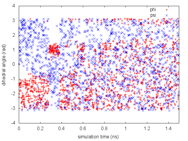
By inspecting Figure belfast-6-metad-fig, we can see that the system is initialized in one of the two metastable states of alanine dipeptide. After a while (t=0.3 ns), the system is pushed by the metadynamics bias potential to visit the other local minimum. As the simulation continues, the bias potential fills the underlying free-energy landscape, and the system is able to diffuse in the entire phase space.
If we use the PLUMED input file described above, the expense of a metadynamics simulation increases with the length of the simulation as one has to evaluate the values of a larger and larger number of Gaussian kernels at every step. To avoid this issue you can store the bias on a grid. In order to use grids, we have to add some additional information to the line of the METAD directive, as follows.
# set up two variables for Phi and Psi dihedral angles
phi: TORSION ATOMS=5,7,9,15
psi: TORSION ATOMS=7,9,15,17
#
# Activate metadynamics in phi and psi
# depositing a Gaussian every 500 time steps,
# with height equal to 1.2 kJoule/mol,
# and width 0.35 rad for both CVs.
# The bias potential will be stored on a grid
# with bin size equal to 0.1 rad for both CVs.
# The boundaries of the grid are -pi and pi, for both CVs.
#
METAD ...
LABEL=metad
ARG=phi,psi
PACE=500
HEIGHT=1.2
SIGMA=0.35,0.35
FILE=HILLS
GRID_MIN=-pi,-pi
GRID_MAX=pi,pi
GRID_SPACING=0.1,0.1
... METAD

# monitor the two variables and the metadynamics bias potential
PRINT STRIDE=10 ARG=phi,psi,metad.bias FILE=COLVAR
The bias potential will be stored on a grid, whose boundaries are specified by the keywords GRID_MIN and GRID_MAX. Notice that you should provide either the number of bins for every collective variable (GRID_BIN) or the desired grid spacing (GRID_SPACING). In case you provide both PLUMED will use the most conservative choice (highest number of bins) for each dimension. In case you do not provide any information about bin size (neither GRID_BIN nor GRID_SPACING) and if Gaussian width is fixed PLUMED will use 1/5 of the Gaussian width as grid spacing. This default choice should be reasonable for most applications.
If we try to run again a metadynamics simulation using the script above in a directory where a COLVAR and HILLS files are already present, PLUMED will create a backup copy of the old files, and run a new simulation. Instead, if we want to restart a previous simulation, we have to add the keyword RESTART to the PLUMED input file (plumed.dat), as follows.
# restart previous simulation
RESTART

# set up two variables for Phi and Psi dihedral angles
phi: TORSION ATOMS=5,7,9,15
psi: TORSION ATOMS=7,9,15,17
#
# Activate metadynamics in phi and psi
# depositing a Gaussian every 500 time steps,
# with height equal to 1.2 kJoule/mol,
# and width 0.35 rad for both CVs.
#
metad: METAD ARG=phi,psi PACE=500 HEIGHT=1.2 SIGMA=0.35,0.35 FILE=HILLS

# monitor the two variables and the metadynamics bias potential
PRINT STRIDE=10 ARG=phi,psi,metad.bias FILE=COLVAR
(see RESTART, TORSION, METAD, and PRINT).
In this way, PLUMED will read the old Gaussian kernels from the HILLS file and append the new information to both COLVAR and HILLS files.
One can estimate the free energy as a function of the metadynamics CVs directly from the metadynamics bias potential. In order to do so, the utility sum_hills should be used to sum the Gaussian kernels deposited during the simulation and stored in the HILLS file.
To calculate the two-dimensional free energy as a function of phi and psi, it is sufficient to use the following command line:
plumed sum_hills --hills HILLS
The command above generates a file called fes.dat in which the free-energy surface as function of phi and psi is calculated on a regular grid. One can modify the default name for the free energy file, as well as the boundaries and bin size of the grid, by using the following options of sum_hills :
--outfile - specify the outputfile for sumhills
--min - the lower bounds for the grid
--max - the upper bounds for the grid
--bin - the number of bins for the grid
--spacing - grid spacing, alternative to the number of bins
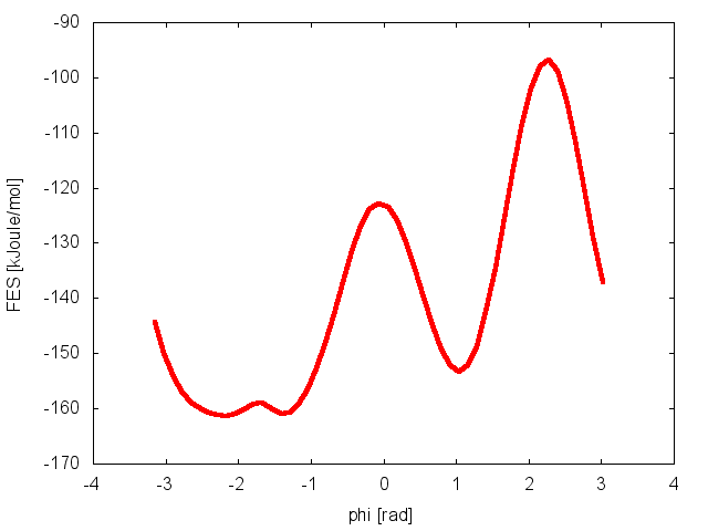
It is also possible to calculate one-dimensional free energies from the two-dimensional metadynamics simulation. For example, if one is interested in the free energy as a function of the phi dihedral alone, the following command line should be used:
plumed sum_hills --hills HILLS --idw phi --kt 2.5
The result should look like this:
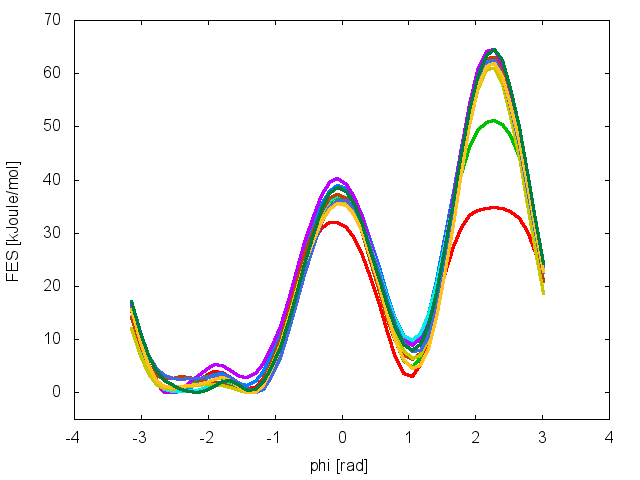
To assess the convergence of a metadynamics simulation, one can calculate the estimate of the free energy as a function of simulation time. At convergence, the reconstructed profiles should be similar, apart from a constant offset. The option –stride should be used to give an estimate of the free energy every N Gaussian kernels deposited, and the option –mintozero can be used to align the profiles by setting the global minimum to zero. If we use the following command line:
plumed sum_hills --hills HILLS --idw phi --kt 2.5 --stride 500 --mintozero
one free energy is calculated every 500 Gaussian kernels deposited, and the global minimum is set to zero in all profiles. The resulting plot should look like the following:
To assess the convergence of the simulation more quantitatively, we can calculate the free-energy difference between the two local minimums in the one-dimensional free energy along phi as a function of simulation time. We can use the bash script analyze_FES.sh to integrate the multiple free-energy profiles in the two basins defined by the following intervals in phi space: basin A, -3<phi<-1, basin B, 0.5<phi<1.5.
./analyze_FES.sh NFES -3.0 -1.0 0.5 1.5 KBT
where NFES is the number of profiles (free-energy estimates at different times of the simulation) generated by the option –stride of sum_hills, and KBT is the temperature in energy units (in this case KBT=2.5).
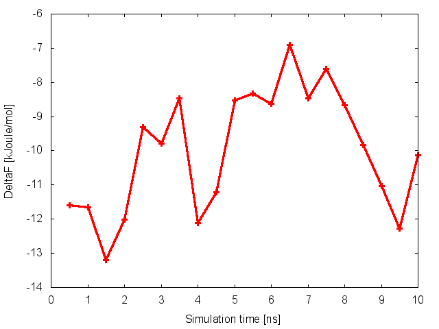
This analysis, along with the observation of the diffusive behavior in the CVs space, suggest that the simulation is converged.
In this exercise, we will run a well-tempered metadynamics simulation on alanine dipeptide in vacuum, using as CVs the two backbone dihedral angles phi and psi. To activate well-tempered metadynamics, we need to add two keywords to the line of METAD, which specifies the bias factor and temperature of the simulation. For the first example, we will try a bias factor equal to 6. Here how the PLUMED input file (plumed.dat) should look like:
# set up two variables for Phi and Psi dihedral angles
phi: TORSION ATOMS=5,7,9,15
psi: TORSION ATOMS=7,9,15,17
#
# Activate metadynamics in phi and psi
# depositing a Gaussian every 500 time steps,
# with height equal to 1.2 kJoule/mol,
# and width 0.35 rad for both CVs.
# Well-tempered metadynamics is activated,
# and the bias factor is set to 6.0
#
metad: METAD ARG=phi,psi PACE=500 HEIGHT=1.2 SIGMA=0.35,0.35 FILE=HILLS BIASFACTOR=6.0 TEMP=300.0

# monitor the two variables and the metadynamics bias potential
PRINT STRIDE=10 ARG=phi,psi,metad.bias FILE=COLVAR
(see TORSION, METAD, and PRINT).
After running the simulation using the instruction described above, we can have a look at the HILLS file. At variance with standard metadynamics, the last two columns of the HILLS file report more useful information. The last column contains the value of the bias factor used, while the last but one the height of the Gaussian, which is rescaled during the simulation following the well-tempered recipe.
#! FIELDS time phi psi sigma_phi sigma_psi height biasf
#! SET multivariate false
#! SET min_phi -pi
#! SET max_phi pi
#! SET min_psi -pi
#! SET max_psi pi
      1.0000     -1.3100    0.0525          0.35            0.35      1.4400      6
      2.0000     -1.4054    1.9742          0.35            0.35      1.4400      6
      3.0000     -1.9997    2.5177          0.35            0.35      1.4302      6
      4.0000     -2.2256    2.1929          0.35            0.35      1.3622      6
If we carefully look at the height column, we will notice that in the beginning the value reported is higher than the initial height specified in the input file, which should be 1.2 kJoule/mol. In fact, this column reports the height of the Gaussian rescaled by the pre-factor that in well-tempered metadynamics relates the bias potential to the free energy. In this way, when we will use sum_hills, the sum of the Gaussian kernels deposited will directly provide the free-energy, without further rescaling needed.
We can plot the time evolution of the CVs along with the height of the Gaussian.
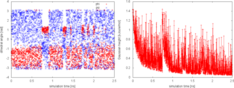
The system is initialized in one of the local minimum where it starts accumulating bias. As the simulation progresses and the bias added grows, the Gaussian height is progressively reduced. After a while (t=0.8 ns), the system is able to escape the local minimum and explore a new region of the phase space. As soon as this happens, the Gaussian height is restored to the initial value and starts to decrease again. In the long time, the Gaussian height becomes smaller and smaller while the system diffuses in the entire CVs space.
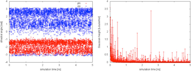
We can now try a different bias factor and see the effect on the simulation. If we choose a bias factor equal to 1.5, we can notice a faster decrease of the Gaussian height with simulation time, as expected by the well-tempered recipe. We will also conclude from the plot below that this bias factor is not large enough to allow for the system to escape from the initial local minimum in the time scale of this simulation.
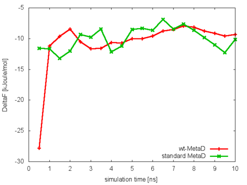
Following the procedure described for standard metadynamics in the previous example, we can estimate the free energy as a function of time and monitor the convergence of the simulations using the analyze_FES.sh script. We will do this for the simulation in which the bias factor was set to 6.0. In this case we will notice that the oscillations observed in standard metadynamics are here damped, and the bias potential converges more smoothly to the underlying free-energy landscape, provided that the bias factor is sufficiently high for the free-energy barriers of the system under study to be crossed.
In this exercise, we will study the effect of neglecting a relavant degree of freedom in the choice of metadynamics CVs. We are going to run a well-tempered metadynamics simulation with the psi dihedral alone as CV, using the following PLUMED input file (plumed.dat):
# set up two variables for Phi and Psi dihedral angles
phi: TORSION ATOMS=5,7,9,15
psi: TORSION ATOMS=7,9,15,17
#
# Activate metadynamics in psi
# depositing a Gaussian every 500 time steps,
# with height equal to 1.2 kJoule/mol,
# and width 0.35 rad.
# Well-tempered metadynamics is activated,
# and the bias factor is set to 10.0
#
metad: METAD ARG=psi PACE=500 HEIGHT=1.2 SIGMA=0.35 FILE=HILLS BIASFACTOR=10.0 TEMP=300.0

# monitor the two variables and the metadynamics bias potential
PRINT STRIDE=10 ARG=phi,psi,metad.bias FILE=COLVAR
(see TORSION, METAD, and PRINT).
Let's look at the HILLS file, in particular at the time serie of the CV psi and of the Gaussian height.
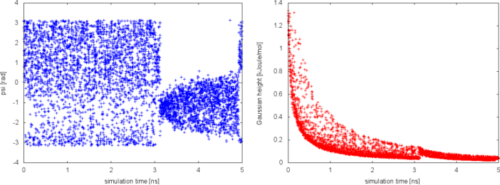
From this plot, we observe a nice diffusive behavior of the CV psi when the Gaussian height is already quite small. This happens until t=3 ns, when the CV seems to be stuck for a while in a small region of the CV space. This behavior is typical of a situation in which a slow variable is not included in the set of CV. When something happens in this hidden degree of freedom, the biased CVs typically cannot access anymore regions of the phase space previously visited. To understand this behavior, we need to visualize the time evolution of both phi and psi stored in the COLVAR file.
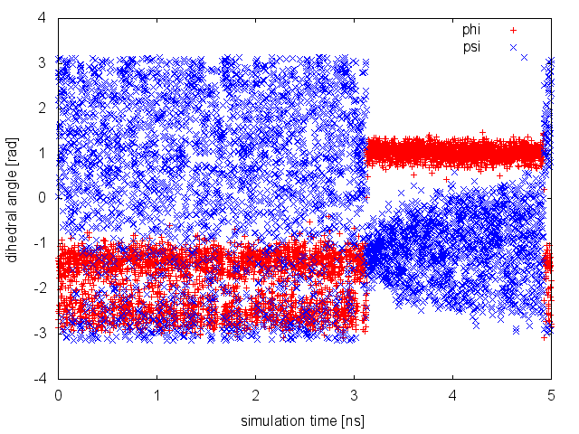
It is clear from the plot above that what happened around t=3 ns is a jump of the neglected, slow degree of freedom phi from one free-energy basin to another. The dynamics of phi is not biased by any potential, so we need to equilibrate this degree of freedom, i.e. to observe multiple transitions from the two basins, before declaring convergence of our simulation. Or alternatively we can add phi to the set of CVs. This example demonstrates how to declare convergence of a well-tempered metadynamics simulation it is necessary but not sufficient to observe: 1) Gaussian kernels with very small height, 2) a diffusive behavior in the CV space (as in the first 3 ns of this example).
What we should do is repeating the simulation multiple times starting from different initial conformations. If in all simulations, we observe a diffusive behavior in the biased CV when the Gaussian height is very small, and we obtain very similar free-energy surfaces, then we can be quite confident that our simulations are converged to the right value. If this is not the case, a manual inspection of the runs can help us identifying the missing slow degrees of freedom to add to the set of biased CVs.
 1.8.14