 |
|
|
| |
|
|
The aim of this tutorial is to train users to perform metadynamics simulations with PLUMED. Error analysis, which is very very important and requires extensive discussions, will be done in a separate tutorial.
Once this tutorial is completed students will be able to:
The TARBALL for this project contains the following files:
This tutorial has been tested on version 2.5.
We have seen that PLUMED can be used to compute collective variables. However, PLUMED is most often use to add forces on the collective variables. To this aim, we have implemented a variety of possible biases acting on collective variables. The complete documentation for all the biasing methods available in PLUMED can be found at the Bias page. In the following we will see how to build an adaptive bias potential with metadynamics. Here you can find a brief recap of the metadynamics theory.
In metadynamics, an external history-dependent bias potential is constructed in the space of a few selected degrees of freedom \( \vec{s}({q})\), generally called collective variables (CVs) [64]. This potential is built as a sum of Gaussian kernels deposited along the trajectory in the CVs space:
\[ V(\vec{s},t) = \sum_{ k \tau < t} W(k \tau) \exp\left( -\sum_{i=1}^{d} \frac{(s_i-s_i({q}(k \tau)))^2}{2\sigma_i^2} \right). \]
where \( \tau \) is the Gaussian deposition stride, \( \sigma_i \) the width of the Gaussian for the \(i\)th CV, and \( W(k \tau) \) the height of the Gaussian. The effect of the metadynamics bias potential is to push the system away from local minima into visiting new regions of the phase space. Furthermore, in the long time limit, the bias potential converges to minus the free energy as a function of the CVs:
\[ V(\vec{s},t\rightarrow \infty) = -F(\vec{s}) + C. \]
In standard metadynamics, Gaussian kernels of constant height are added for the entire course of a simulation. As a result, the system is eventually pushed to explore high free-energy regions and the estimate of the free energy calculated from the bias potential oscillates around the real value. In well-tempered metadynamics [8], the height of the Gaussian is decreased with simulation time according to:
\[ W (k \tau ) = W_0 \exp \left( -\frac{V(\vec{s}({q}(k \tau)),k \tau)}{k_B\Delta T} \right ), \]
where \( W_0 \) is an initial Gaussian height, \( \Delta T \) an input parameter with the dimension of a temperature, and \( k_B \) the Boltzmann constant. With this rescaling of the Gaussian height, the bias potential smoothly converges in the long time limit, but it does not fully compensate the underlying free energy:
\[ V(\vec{s},t\rightarrow \infty) = -\frac{\Delta T}{T+\Delta T}F(\vec{s}) + C. \]
where \( T \) is the temperature of the system. In the long time limit, the CVs thus sample an ensemble at a temperature \( T+\Delta T \) which is higher than the system temperature \( T \). The parameter \( \Delta T \) can be chosen to regulate the extent of free-energy exploration: \( \Delta T = 0\) corresponds to standard MD, \( \Delta T \rightarrow\infty\) to standard metadynamics. In well-tempered metadynamics literature and in PLUMED, you will often encounter the term "bias factor" which is the ratio between the temperature of the CVs ( \( T+\Delta T \)) and the system temperature ( \( T \)):
\[ \gamma = \frac{T+\Delta T}{T}. \]
The bias factor should thus be carefully chosen in order for the relevant free-energy barriers to be crossed efficiently in the time scale of the simulation. Additional information can be found in the several review papers on metadynamics [63] [9] [101] [26]. To learn more: Summary of theory
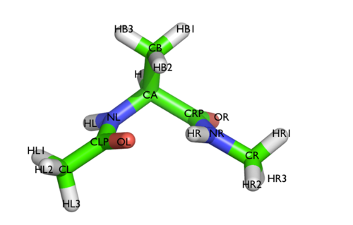
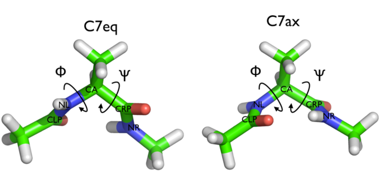
We will play with a toy system, alanine dipeptide simulated in vacuo using the AMBER99SB-ILDN force field (see Fig. lugano-3-ala-fig). This rather simple molecule is useful to understand data analysis and free-energy methods. This system is a nice example because it presents two metastable states separated by a high free-energy barrier. It is conventional use to characterize the two states in terms of Ramachandran dihedral angles, which are denoted with \( \Phi \) and \( \Psi \) in Fig. lugano-3-transition-fig .
In this exercise we will setup and perform a well-tempered metadynamics run using the backbone dihedral \( \phi \) as collective variable. During the calculation, we will also monitor the behavior of the other backbone dihedral \( \psi \).
Here you can find a sample plumed.dat file that you can use as a template. Whenever you see an highlighted FILL string, this is a string that you should replace.
# vim:ft=plumed
MOLINFO STRUCTURE=diala.pdb
# Compute the backbone dihedral angle phi, defined by atoms C-N-CA-C
# you might want to use MOLINFO shortcuts
phi: TORSION ATOMS=__FILL__
# Compute the backbone dihedral angle psi, defined by atoms N-CA-C-N
psi: TORSION ATOMS=__FILL__

# Activate well-tempered metadynamics in phi
metad: __FILL__ ARG=__FILL__ ...
# Deposit a Gaussian every 500 time steps, with initial height equal to 1.2 kJ/mol
  PACE=500 HEIGHT=1.2
# the bias factor should be wisely chosen
  BIASFACTOR=__FILL__
# Gaussian width (sigma) should be chosen based on CV fluctuation in unbiased run
  SIGMA=__FILL__
# Gaussians will be written to file and also stored on grid
  FILE=HILLS GRID_MIN=-pi GRID_MAX=pi
...

# Print both collective variables and the value of the bias potential on COLVAR file
PRINT ARG=__FILL__ FILE=COLVAR STRIDE=10
The syntax for the command METAD is simple. The directive is followed by a keyword ARG followed by the labels of the CVs on which the metadynamics potential will act. The keyword PACE determines the stride of Gaussian deposition in number of time steps, while the keyword HEIGHT specifies the height of the Gaussian in kJ/mol. For each CVs, one has to specify the width of the Gaussian by using the keyword SIGMA. Gaussian will be written to the file indicated by the keyword FILE.
In this example, the bias potential will be stored on a grid, whose boundaries are specified by the keywords GRID_MIN and GRID_MAX. Notice that you can provide either the number of bins for every collective variable (GRID_BIN) or the desired grid spacing (GRID_SPACING). In case you provide both PLUMED will use the most conservative choice (highest number of bins) for each dimension. In case you do not provide any information about bin size (neither GRID_BIN nor GRID_SPACING) and if Gaussian width is fixed, PLUMED will use 1/5 of the Gaussian width as grid spacing. This default choice should be reasonable for most applications.
Once your plumed.dat file is complete, you can run a 10-ns long metadynamics simulations with the following command
> gmx mdrun -s topol.tpr -nsteps 5000000 -plumed plumed.dat
During the metadynamics simulation, PLUMED will create two files, named COLVAR and HILLS. The COLVAR file contains all the information specified by the PRINT command, in this case the value of the CVs every 10 steps of simulation, along with the current value of the metadynamics bias potential. We can use gnuplot to visualize the behavior of the CV during the simulation, as reported in the COLVAR file:
gnuplot> p "COLVAR" u 1:2
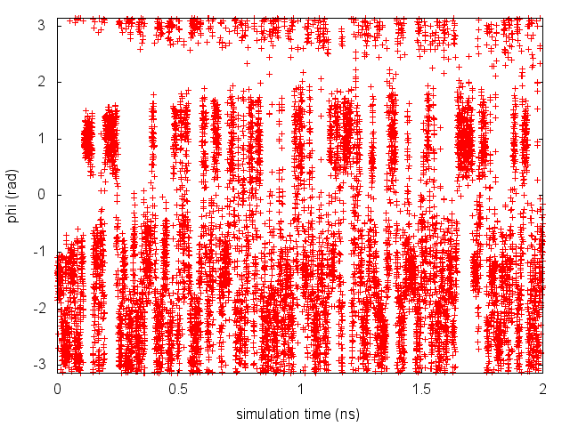
By inspecting Figure lugano-3-phi-fig, we can see that the system is initialized in one of the two metastable states of alanine dipeptide. After a while (t=0.1 ns), the system is pushed by the metadynamics bias potential to visit the other local minimum. As the simulation continues, the bias potential fills the underlying free-energy landscape, and the system is able to diffuse in the entire phase space.
The HILLS file contains a list of the Gaussian kernels deposited along the simulation. If we give a look at the header of this file, we can find relevant information about its content:
#! FIELDS time phi sigma_phi height biasf
#! SET multivariate false
#! SET min_phi -pi
#! SET max_phi pi
The line starting with FIELDS tells us what is displayed in the various columns of the HILLS file: the simulation time, the instantaneous value of \( \phi \), the Gaussian width and height, and the bias factor. We can use the HILLS file to visualize the decrease of the Gaussian height during the simulation, according to the well-tempered recipe:
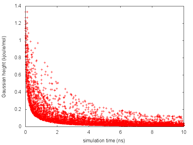
If we look carefully at the scale of the y-axis, we will notice that in the beginning the value of the Gaussian height is higher than the initial height specified in the input file, which should be 1.2 kJ/mol. In fact, this column reports the height of the Gaussian scaled by the pre-factor that in well-tempered metadynamics relates the bias potential to the free energy.
One can estimate the free energy as a function of the metadynamics CVs directly from the metadynamics bias potential. In order to do so, the utility sum_hills should be used to sum the Gaussian kernels deposited during the simulation and stored in the HILLS file.
To calculate the free energy as a function of \( \phi \), it is sufficient to use the following command line:
plumed sum_hills --hills HILLS
The command above generates a file called fes.dat in which the free-energy surface as function of \( \phi \) is calculated on a regular grid. One can modify the default name for the free energy file, as well as the boundaries and bin size of the grid, by using the following options of sum_hills :
--outfile - specify the outputfile for sumhills
--min - the lower bounds for the grid
--max - the upper bounds for the grid
--bin - the number of bins for the grid
--spacing - grid spacing, alternative to the number of bins
The result should look like this:
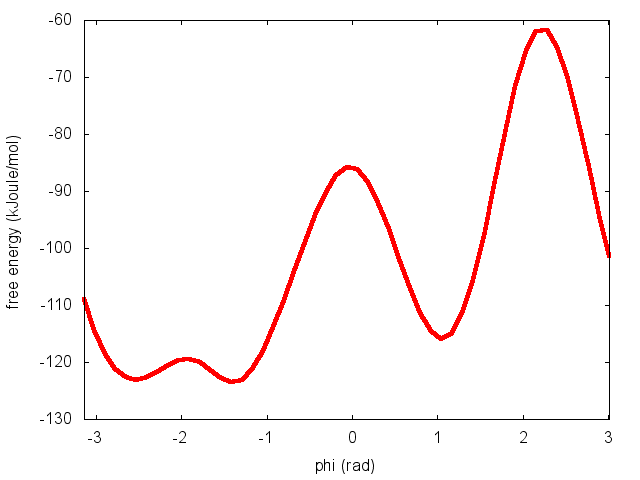
To assess the convergence of a metadynamics simulation, one can calculate the estimate of the free energy as a function of simulation time. At convergence, the reconstructed profiles should be similar. The option --stride should be used to give an estimate of the free energy every N Gaussian kernels deposited, and the option --mintozero can be used to align the profiles by setting the global minimum to zero. If we use the following command line:
plumed sum_hills --hills HILLS --stride 100 --mintozero
one free energy is calculated every 100 Gaussian kernels deposited, and the global minimum is set to zero in all profiles. The resulting plot should look like the following:
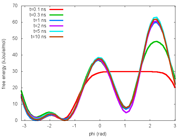
These two qualitative observations:
suggest that the simulation most likely converged.
The bias factor allows you to choose how extensive your sampling of the CV space will be. If you choose it too large, you will explore a large reason of the CV space and your simulation will take more time to converge. If you choose it too small, you will not be able to cross the barriers you are interested in.
Try to run your simulation with different values of the bias factor. Going low to anything that is greater than 1 should give meaningful results, although if the chosen value is too low the system will only explore a limited portion of the space.
Which is the minimum value of the bias factor that allows you to see, in the simulated time, transitions between the two relevant minima?
In the previous exercise we biased \(\phi\) and compute the free energy as a function of the same variable. Many times you want to decide which variable you want to analyze after having performed a simulation. In order to do so you must reweight your simulation.
There are multiple ways to reweight a metadynamics simulations. In order to calculate these weights, we can use either of these two approaches:
1) Weights are calculated by considering the time-dependence of the metadynamics bias potential [103];
2) Weights are calculated using the metadynamics bias potential obtained at the end of the simulation and assuming a constant bias during the entire course of the simulation [24].
In this exercise we will use the umbrella-sampling-like reweighting approach (Method 2). In order to compute the weights we will use the driver tool.
First of all, prepare a plumed_reweight.dat file that is identical to the one you used for running your simulation but add the keyword RESTART=YES to the METAD command. This will make this action behave as if PLUMED was restarting. It will thus read the already accumulated hills and continue adding more. In addition, set hills height to zero and the pace to a large number. This will actually avoid adding new hills (and even if they are added they will have zero height). Finally, change the PRINT statement so that you write every frame (STRIDE=1) and that, in addition to phi and psi, you also write `metad.bias.
__FILL__ # here goes the definitions of the CVs

# Activate well-tempered metadynamics in phi
metad: __FILL__ ARG=__FILL__ ...
# Deposit a Gaussian every 500 time steps, with initial height equal to 1.2 kJ/mol
  PACE=10000000 HEIGHT=0.0 # <- this is the new stuff!
# the bias factor should be wisely chosen
  BIASFACTOR=__FILL__
# Gaussian width (sigma) should be chosen based on CV fluctuation in unbiased run
  SIGMA=__FILL__
# Gaussians will be written to file and also stored on grid
  FILE=HILLS GRID_MIN=-pi GRID_MAX=pi
# Say that METAD should be restarting
  RESTART=YES # <- this is the new stuff!
...

PRINT ARG=phi,psi,metad.bias FILE=COLVAR STRIDE=1  # <- also change this one!
Then run the driver using this command
> plumed driver --ixtc traj_comp.xtc --plumed plumed.dat --kt 2.5
Notice that you have to specify the value of \(k_BT\) in energy units. While running your simulation this information was taken from the MD code.
As a result, PLUMED will produce a new COLVAR file with an additional column. The beginning of the file should look like this:
#! FIELDS time phi psi metad.bias
#! SET min_phi -pi
#! SET max_phi pi
#! SET min_psi -pi
#! SET max_psi pi
 0.000000 -1.497988 0.273498 110.625670
 1.000000 -1.449714 0.576594 110.873141
 2.000000 -1.209587 0.831417 109.742353
 3.000000 -1.475975 1.279726 110.752327
The last column will give as, in energy units, the logarithm of the weight of each frame. You can easily obtain the weight of each frame using the expression \(w\propto\exp\left(\frac{V(s)}{k_BT}\right)\). You might want to read the COLVAR file in python and compute a weighted histogram.
If you want PLUMED to do the histograms for you, you can just add the following lines that you learned in Lugano tutorial: Using restraints to the plumed input file:
as: REWEIGHT_BIAS ARG=__FILL__

hhphi: HISTOGRAM ARG=phi STRIDE=50 GRID_MIN=-pi GRID_MAX=pi GRID_BIN=600 BANDWIDTH=0.1 LOGWEIGHTS=as
hhpsi: HISTOGRAM ARG=psi STRIDE=50 GRID_MIN=-pi GRID_MAX=pi GRID_BIN=600 BANDWIDTH=0.1 LOGWEIGHTS=as
ffphi: CONVERT_TO_FES GRID=hhphi
ffpsi: CONVERT_TO_FES GRID=hhpsi

DUMPGRID GRID=ffphi FILE=ffphi.dat
DUMPGRID GRID=ffpsi FILE=ffpsi.dat
and plot the result using gnuplot.
gnuplot> p "ffphi.dat"
gnuplot> p "ffpsi.dat"
Alanine dipeptide is often considered as a too-simple system to understand the typical problems that one will then see in real systems. This is very much not true! We will here see how to make the exercise arbitrarily difficult, to the point that metadynamics will not work anymore.
The difficult case of metadynamics is when there are variables that (a) are orthogonal to the biased ones and (b) exhibit large energy barriers. The first point implies that when you flatten the distribution of the biased collective variables you are not accelerating the sampling of the orthogonal variables. The second point implies that those variable will take a lot of time to explore different metastable states.
Often these variables are not known and they are thus called "hidden variables". In the case of alanine dipeptide, we can easily add a barrier on \(\Psi\) with some additional PLUMED command. We will add a Gaussian barrier centered at \(\Psi=0.5\). To do so, add to the PLUMED input file that you prepared for the first exercise (that is: biasing \(\Phi\) alone) the following lines
# first shift the psi variable.
# setting the new periodicity to -pi,pi will make sure that the barrier
# is a continuous function of the coordinates
shift1:   CUSTOM ARG=psi   FUNC=x-0.5 PERIODIC=-pi,pi
shift2:   CUSTOM ARG=psi   FUNC=x+2.5 PERIODIC=-pi,pi
# then compute the barrier energy.
# this would be a Gaussian with wifth 0.3. You can pick the height as you like
barrier:  CUSTOM ARG=shift1,shift2 FUNC=__FILL__*exp(-0.5*x^2/0.2^2)+__FILL__*exp(-0.5*y^2/0.2^2) PERIODIC=NO
# then add the barrier to the total energy of the system.
BIASVALUE ARG=barrier
Something high like 25 kj/mol should create a significant difficulty. Notice that this means a barrier 10 \(k_BT\) high in a direction that is not being biased.
You should see something like this
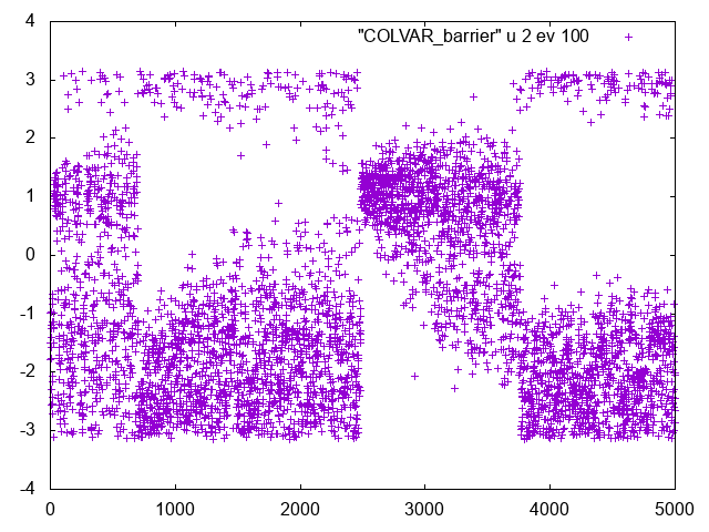
If you look at this series you will clearly see that there are clear changes in the Phi dynamics. If you look at Psi dynamics you should be able to see that these changes correspond to transitions in Psi.
This is an indication that an important slow variable is missing.
Find the minimum value of the barrier required for the simulation not to converge in the simulated timescale.
In summary, in this tutorial you should have learned how to use PLUMED to:
 1.8.14