 |
|
|
| |
|
|
Consider the two overlain protein structures that are shown in the figure below.
Can you see the difference between these two structures? Can you think of a collective variable that could be used to study the substantial change in structure?
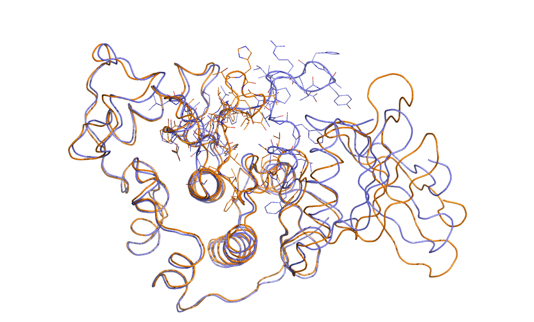
Your answers to the questions posed above are hopefully: yes I can see the difference between the two structures - the upper loop is radically different in the two cases - and no I have absolutely no idea as to how to create a collective variable that might be used to study the change in structure.
These answers are interesting as they cut to the very heart of what is interesting about biomolecular systems. In fact this difficulty is one of the reasons why such systems are so widely studied. If you think for a moment about solid state systems any transition usually involves a substantial change in symmetry.
Low energy configurations are usually high symmetry while higher energy configurations have a low symmetry. This makes it easy to design collective variables to study solid state transitions - you simply measure the degree of symmetry in the system (see Belfast tutorial: Steinhardt Parameters). In biomolecular systems by contrast the symmetry does not change substantially during a folding transition. The unfolded state has a low symmetry but the folded state also has a low symmetry, which is part of the reason that it is so difficult to find the folded state from the amino acid sequence alone.
With all this in mind the purpose of this tutorial is to learn about how we can design collective variables that can be used to study transitions between different states of these low-symmetry systems. In particular, we are going to learn how we can design collective variables that describe how far we have progressed along some pathway between two configurations with relatively low symmetry. We will in most of this tutorial study how these coordinates work in a two-dimensional space as this will allow us to visualize what we are doing. Hopefully, however, you will be able to use what you learn from this tutorial to generalize these ideas so that you can use PATH and PCAVARS in higher-dimensional spaces.
Once this tutorial is completed students will:
The tarball for this project contains the following files:
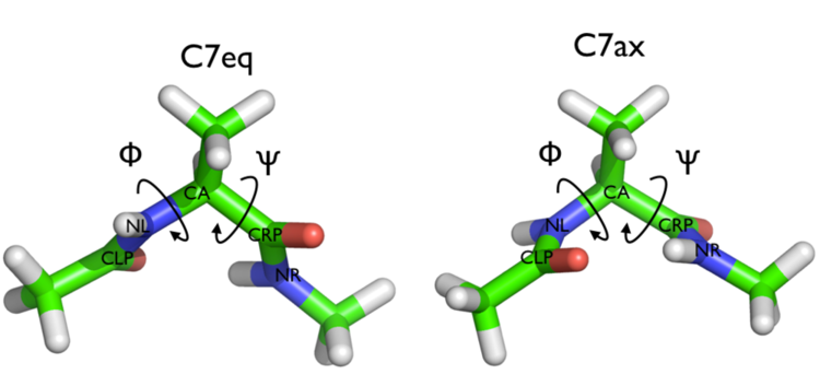
In this tutorial we are going to be considering a conformational transition of alanine dipeptide. In particular we are going to be considering the transition between the two conformers of this molecule shown below:
Alanine dipeptide is a rather well-studied biomolecule (in fact it is an over studied molecule!). It is well known that you can understand the inter-conversion of the two conformers shown above by looking at the free energy surface as a function of the \(\phi\) and \(\psi\) Ramachandran angles as shown below:

In this tutorial we are not going to use these coordinates to study alanine dipeptide. Instead we are going to see if we can find a single collective variable that can distinguish between these two states.
Consider the free energy surface shown in figure marvel-2-rama-fig. It is clear that either the \(\phi\) ( \(x\)-axis) or the \(\psi\) ( \(y\)-axis) angle of the molecule can be used to distinguish between the two configurations shown in figure marvel-2-transition-fig. Having said that, however, given the shape of landscape and the associated thermal fluctuations we would expect to see in the values of these angles during a typical simulation, it seems likely that \(\phi\) will do a better job at distinguishing between the two configurations. \(\psi\) would most likely be a bad coordinate as when the molecule is in the \(C_7eq\) configuration the \(\psi\) angle can fluctuate to any value with only a very small energetic cost. If we only had information on how the \(\psi\) angle changed during a simulation we would thus struggle to distinguish a transition to the \(C_7ax\) configuration from a thermal fluctuations. It has been shown that metadynamics simulations that use just the \(\phi\) angle as a collective variable can effectively drive the system from the \(C_7ax\) configuration to the \(C_7eq\) configuration. We will not repeat these calculations here but will instead use driver to determine how the values of \(\phi\) and \(\psi\) change as we move between along the transition path that connects the \(C_7ax\) configuration to the \(C_7eq\) state.
t1: TORSION ATOMS=2,4,6,9
t2: TORSION ATOMS=4,6,9,11
PRINT ARG=t1,t2 FILE=colvar
Lets run this now on trajectory that describes the transition from the \(C_7ax\) configuration to the \(C_7eq\) configuration. To run this calculation copy the input file above into a file called plumed.dat and run the command below:
plumed driver --mf_pdb transformation.pdb
Try plotting each of the two torsional angles in this file against time in order to get an idea of how good a job each one of these coordinates at distinguishing between the various configurations along the pathway connecting the \(C_7ax\) and \(C_7eq\) configurations. What you will see is that in both cases the CV does not increase/decrease monotonically as the transition progresses.
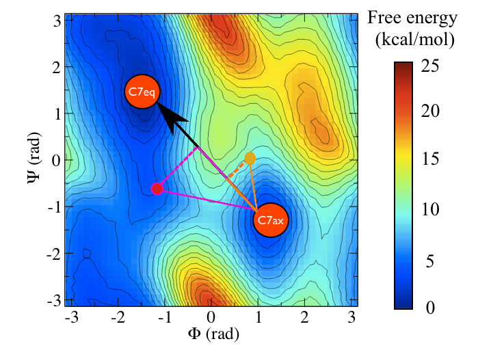
We can perhaps come up with a better coordinate that incorporates changes in both \(\phi\) and \(\psi\) by using the coordinate illustrated in the figure below.
We can even use PLUMED to calculate this coordinate by using the input shown below:
t1: TORSION ATOMS=2,4,6,9
t2: TORSION ATOMS=4,6,9,11
tc: COMBINE ARG=t1,t2 COEFFICIENTS=2.621915,-2.408714 PERIODIC=NO
PRINT ARG=t1,t2,tc FILE=colvar
Try calculating the values of the above collective variables for each of the configurations in the transformation.pdb file by using the command that was given earlier.
Notice that what we are using here are some well known results on the dot product of two vectors here. Essentially if the values of the Ramachandran angles in the \(C_7eq\) configuration are \((\phi_1,\psi_1)\) and the Ramachandran angles in the \(C_7ax\) configuration are \((\phi_2,\psi_2)\). If our instantaneous configuration is \((\phi_3,\psi_3)\) we can thus calculate the following projection on the vector connecting the \(C_7eq\) state to the \(C_7ax\) state:
\[ s = (\phi_2 - \phi_1).(\phi_3 - \phi_1) + (\psi_2 - \psi_1).(\psi_3 - \psi_1) \]
which is just the dot product between the vector connecting the point \((\phi_1,\psi_1)\) to \((\phi_2,\psi_2)\) and the vector connecting the point \((\phi_1,\psi_1)\) to \((\phi_3,\psi_3)\). If we call these two vectors \(\mathbf{v}_1\) and \(\mathbf{v}_2\) we can write this dot product as:
\[ \mathbf{v}_1 \cdot \mathbf{v}_2 = | \mathbf{v}_1 | | \mathbf{v}_2 | cos( \alpha ) \]
where \(| \mathbf{v}_1 |\) and \(| \mathbf{v}_2 |\) are the magnitudes of our two vectors and where \(\alpha\) is the angle between the two of them. Elementary trigonometry thus tells us that if \(\mathbf{v}_1\) is a unit vector (i.e. if it has magnitude 1) the dot product is thus equal to the projection of the vector \(\mathbf{v}_2\) on \(\mathbf{v}_2\) as shown in figure pca-figure.
This is an useful idea. In fact it is the basis of the PCAVARS collective variable that is implemented in PLUMED so we can (almost) calculate the projection on this vector by using the input shown below:
t1: TORSION ATOMS=2,4,6,9
t2: TORSION ATOMS=4,6,9,11
p: PCAVARS REFERENCE=angle-pca-reference.pdb TYPE=EUCLIDEAN
PRINT ARG=t1,t2,p.* FILE=colvar
We cannot, however, do this in practice (we also shouldn't really use the previous input either) as the TORSION angles that we use to define our vectors here are periodic. In this next section we will thus look at how we can avoid this problem of periodicity by working in a higher dimensional space.
In the previous section I showed how we can use the projection of a displacement on a vector as a collective variable. I demonstrated this in a two dimensional space as this makes it easy to visualize the vectors involved. We are not forced to work with two dimensional vectors, however. We can instead find the vector that connects the \(C_7eq\) and \(C_7ax\) states in some higher dimensional space and project our current coordinate on that particular vector. In fact we can even define this vector in the space of the coordinates of the atoms. In other words, if the 3 \(N\) coordinate of atomic positions is \(\mathbf{x}^{(1)}\) for the \(C_7eq\) configuration and \(\mathbf{x}^{(2)}\) for the \(C_7ax\) configuration and if the instantaneous configuration of the atoms is \(\mathbf{x}^{(3)}\) we can use the following as a CV:
\[ s = \sum_{i=1}^{3N} (x^{(2)}_i - x^{(1)}_i ) (x^{(3)}_i - x^{(1)}_i ) \]
where the sum here runs over the \(3N\)-dimensional vector that defines the positions of the \(N\) atoms in the system. This is what (in a manner of speaking - I will return to this point momentarily) is calculated by this PLUMED input:
t1: TORSION ATOMS=2,4,6,9
t2: TORSION ATOMS=4,6,9,11
p: PCAVARS REFERENCE=pca-reference.pdb TYPE=OPTIMAL
PRINT ARG=t1,t2,p.* FILE=colvar
Use this input to analyze the set of configurations that are in the transformation.pdb file.
Let's now look further at the caveat that I alluded to before we ran the calculations. I stated that we are only calculating:
\[ s = \sum_{i=1}^{3N} (x^{(2)}_i - x^{(1)}_i ) (x^{(3)}_i - x^{(1)}_i ) \]
in a manner of speaking. The point is that we would not want to calculate exactly this quantity because the vectors of displacements that are calculated in this way includes both rotational and translational motion. This is a problem as the majority of the change in moving from the \(C_7ax\) configuration shown in figure marvel-2-transition-fig to the \(C_7eq\) configuration shown in figure marvel-2-transition-fig comes from the translation of all the atoms. To put this another way if I had, in figure marvel-2-transition-fig, shown two images of the \(C_7ax\) configuration side by side the displacement in the positions of the atoms in those two structures would be similar to the displacement of the atoms in marvel-2-transition-fig as as the majority of the displacement in the vector of atomic positions comes about because I have translated all the atoms in the molecule rightwards by a fixed amount. I can, however, remove these translational displacements from consideration when calculating these vectors. In addition, I can also remove any displacements due rotation in the frame of reference of the molecule. If you are interested in how this is done in practice you can read about it on the manual page about the RMSD collective variable. For what concerns us here, however, all we need to know is that when we use the OPTIMAL metric we are calculating a vector which tells us how far the atoms have been displaced in moving from structure A to structure B in a way that excludes any displacements due to translation of the center of mass of the molecule or any displacements that occur due to rotation of the Cartesian frame.
In the previous sections I have been rather loose when talking about better and worse collective variables in that I have not been clear in my distinction between what makes a collective variable good and what makes a collective variable bad. In this section I thus want to discuss one method that we can use to judge the quality of a collective variable. This method involves calculating the so called isocommittor. The essential notion behind this technique is that there will be a saddle point between the two states of interest (the \(C_7ax\) and \(C_7eq\) configurations in our alanine dipeptide example). If the free energy is plotted as a function of a good collective variable the location of this dividing surface - the saddle point - will appear as a maximum.
Lets suppose that we now start a simulation with the system balanced precariously on this maximum. The system will, very-rapidly, fall off the maximum and move towards either the left or the right basin. Furthermore, if this maximum provides a good representation of the location of the transition state ensemble - in other words if the position of maximum in the low-dimensional free energy surface tells us something about the structure in the transition state ensemble - then 50% of trajectories started from this point will fall to the left and 50% will fall to the right. If by contrast the maximum in the free energy surface does not represent the location of the transition state well then there will be an imbalance between the number of trajectories that move rightwards and the number that move leftwards.
We can think of this business of the isocommittor one further way, however. If in the vicinity of the transition state between the two basins the collective variable is perpendicular to the surface separating these two states half of the trajectories that start from this configuration will move to the left in CV space while the other half will move to the right. If the dividing surface and the CV are not perpendicular in the vicinity of the transition state, however, there will be an imbalance between the number of trajectories that move rightwards and the number of trajectories that move leftwards. We can thus determine the goodness of a collective variable by shooting trajectories from what we believe is the transition state and examining the number of trajectories that move into the left and right basins.
Lets make all this a bit more concrete by looking at how we might calculate the isocommittor by using some of the collective variables we have introduced in this exercise. You will need to go into the directory in the tar ball that you downloaded that is called PCA-isocommittor. In this directory you will find a number of files that will serve as input to gromacs 5 and PLUMED. You thus need to ensure that you have an installed version of gromacs 5 patched with PLUMED on your computer in order to perform this exercise. In addition to these input files you will find a bash script called script.sh, which we are going to use in order to set of a large number of molecular dynamics simulations. If you open script.sh you will find the following lines near the top:
GROMACS_BIN=/Users/gareth/MD_code/gromacs-5.1.1/build/bin
GROMACS=$GROMACS_BIN/gmx
source $GROMACS_BIN/GMXRC.bash
These will need to be adjusted so that the GROMACS_BIN variable points at the bin directory of the gromacs build on your computer. Once you have made this modification though you can run the calculation by issuing the following command in the PCA-isocommittor directory:
./script.sh
This command submits 50 molecular dynamics simulations that all start from a configuration that lies between the \(C_7eq\) and \(C_7ax\) configurations of alanine dipeptide. In addition, this command also generates some scripts that allow us to visualize how the \(\phi\), \(\psi\) and PCA coordinates that we introduced in the previous sections change during each of these 50 simulations. If you load gnuplot and issue the command:
load "script_psi.gplt"
you see how \(\psi\) changes during the course of the 50 simulations. Similarly the gnuplot command:
load "script_phi.gplt"
will show how how \(\phi\) changes during the course of the 50 simulations and:
load "script_pca.gplt"
gives you the information on the PCA coordinates. If you look at the \(\psi\) and PCA data first you can see clearly that it is very difficult to distinguish the configurations that moved to the \(C_7eq\) basin from the trajectories that moved to the \(C_7ax\) basin. By contrast if you look at the data on the \(\phi\) angles you can indeed use these plots to distinguish the trajectories that moved to \(C_7eq\) from the trajectories that moved to \(C_7ax\). It is abundantly clear, however, that the number of trajectories that moved to \(C_7eq\) is not equal to the number of trajectories that moved to \(C_7ax\). This CV, therefore, is not capturing the transition state ensemble.
One thing you will have seen from these examples is that the PCAVARS coordinate that were introduced in the previous sections provides an extremely poor model for the transition state ensemble. The value of the isocommittor at the maximum for both of these variables is not at all close to 50%. In fact the CV is not even particularly good at capturing the difference between these two states. If you look at the free energy surface shown below it is perhaps clear why.
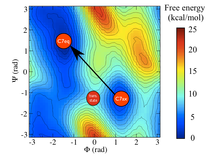
You can see the location of the saddle point between these two states in this surface and it is very clear that the vector connecting the \(C_7eq\) state to the \(C_7ax\) state does not pass through this point. In fact it would be extremely fortuitous if a vector connecting an initial state and a final state also passed through the intermediate transition state between them. We can, after all, define the equation of straight line (a vector) if we are given only two points on it. In the next section we are thus going to see how we can resolve this problem by introducing a non-linear (or curvilinear) coordinate.
Consider the black path that connects the \(C_7ax\) and \(C_7eq\) states in the free energy shown below:
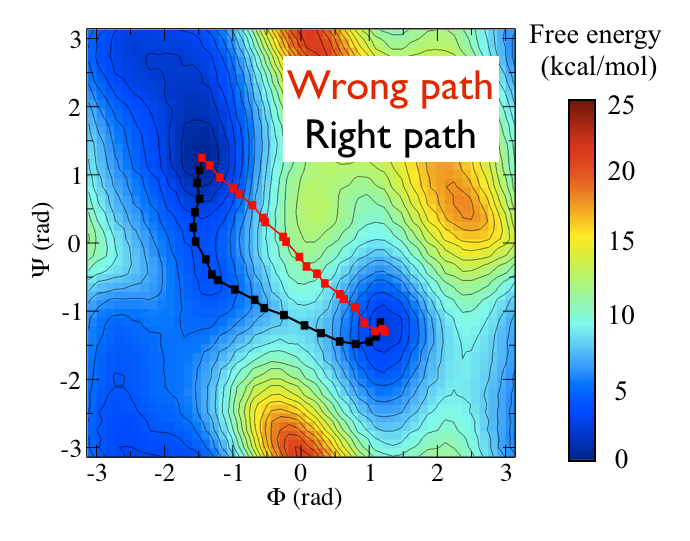
This black pathways appears to be the "perfect" coordinate for modelling this conformational transition as it passes along the lowest energy pathway that connects the two states and because it thus passes over the lowest saddle point that lies between them. We can calculate such a coordinate with PLUMED by using the input file below (I will return to the mathematical details of how this works momentarily)
path: PATH REFERENCE=path-reference.pdb TYPE=OPTIMAL LAMBDA=15100.
PRINT ARG=* STRIDE=2 FILE=colvar FMT=%12.8f
Lets thus use this input and run an isocommittor analysis using the location of the maximum in this coordinate as the start point for all our trajectories. Everything you need to do this analysis is in the PATH-isocommittor directory. Once again you will find that there is a script.sh bash script inside this directory, which, as in the previous section, you can use to run a large number of molecular dynamics simulation. Furthermore, similarly to the last section you will need to begin this exercise by modifying the location of path to gromacs within this script. Once you have made this modification submit your molecular dynamics jobs by issuing the command:
./script.sh
You can then plot the data output using gnuplot and the command:
load "script_path.gplt"
Unlike what we saw for the PCAVARS variables in the previous section we find that it is easy to use these PATH variables to distinguish those configurations that moved to \(C_7ax\) from those that moved to \(C_7eq\). Having said that, however, we still have a large imbalance between the number of trajectories that move rightwards and the number that move leftwards. We are thus still a long way from unambiguously identifying the location of the transition state ensemble for this system.
Let's now take a moment to discuss the mathematics of these coordinates, which is not so complicated if we think about what they do through an analogy. Suppose that you were giving your friend instructions as to how to get to your house and lets suppose these instructions read something like this:
The house is on the corner by the garage.
If you think about these instructions in the abstract what you have is a set of way markers (the item I have put in bold) in a particular order. The list of way markers is important as is the order they appear in in the instructions so we incorporate both these items in the PATH coordinates that we have just used to study the transition between the transition between \(C_7eq\) and \(C_7ax\). In these coordinates the way markers are a set of interesting points in a high dimensional space. In other words, these are like the configurations of \(C_7eq\) and \(C_7ax\) that we used in the previous sections when talking about PCAVARS. Each of these configurations lies along the path connecting \(C_7eq\) and \(C_7ax\) and, as in the directions example above, one must pass them in a particular order in order to pass between these two conformations. The final CV that we have used above is thus:
\[ S(X)=\frac{\sum_{i=1}^{N} i\ \exp^{-\lambda \vert X-X_i \vert }}{ \sum_{i=1}^{N} \exp^{-\lambda \vert X-X_i \vert } } \]
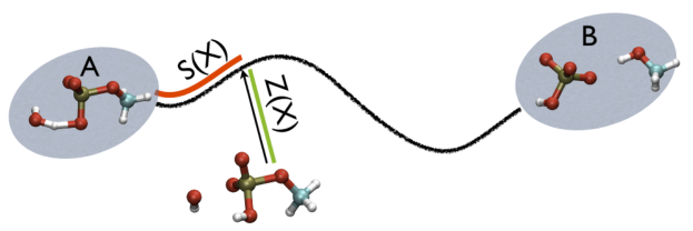
In this expression \(\vertX-X_i\vert\) is the distance between the instantaneous coordinate of the system, \(X\), in the high-dimensional space and \(X_i\) is the coordinate of the \(i\)th way mark in the path. The largest exponential in the sum that appears in the numerator and the denominator will thus be the one that corresponds to the point that is closest to where the system currently lies. In other words, \(S(X)\), measures the position on a (curvilinear) path that connects two states of interest as shown in red in the figure below:
You may reasonably ask what the purpose these PATH collective variables variables serve given that in this case they seem to do no better than \(\phi\) when it comes to the tests we have performed on calculating the isocommittor. To answer this question we are going to run one final set of isocommittor simulations. The input for these calculations are in the directory called 2CV-isocommittor. Once again you will find that there is a script.sh bash script inside this directory, which, as in the previous section, you can use to run a large number of molecular dynamics simulation. Furthermore, similarly to the last section you will need to begin this exercise by modifying the location of path to gromacs within this script. Once you have made this modification submit your molecular dynamics jobs by issuing the command:
./script.sh
You can then plot the data output using gnuplot and the commands:
load "script_pca.gplt"
and
load "script_path.gplt"
What is plotted by these commands is slightly different from what was plotted in the previous exercises where we calculated the isocommittor.
Instead of plotting the value of the CV against simulation time the above commands plot the values that 2CVs take during the simulation. The script called script_path.gplt plots the value of the \(S(X)\) collective variable on the x-axis and the value of the following quantity on the y-axis:
\[ Z(X)=-\frac{1}{\lambda}\log (\sum_{i=1}^{N} \ \exp^{-\lambda \vert X-X_i \vert }) \]
What this quantity measures is shown in green in the figure marvel-2-ab-sz-fig. Essentially it measures the distance between the instantaneous configuration the system finds itself in and the path that is marked out using the way markers. If you plot the data using script_path.gplt what you thus see is that the system never moves very far from the path that is defined using the PATH command. In short the system follows this path from the transition state back to either the \(C_7eq\) or \(C_7ax\) configuration.
We can calculate a quantity similar to \(Z(X)\) for the PCAVARS collective variables. Furthermore, when we plot the data we have generated using this exercise using script_pca.gplt the value this quantity takes is shown plotted against the instantaneous value of the PCAVARS collective variable. If you compare this graph with what was obtained when you plotted the output from PATH above you see that the system has moved very far from the PCAVARS coordinate.
This exercise illustrates the strength of these PATH collective variables. We can use a PATH to monitor how a large number of coordinates change during a chemical transition. Furthermore, we can use \(Z(X)\) to measure how much real trajectories deviate from our PATH and thus have a quantitative measure of how well our PATH represents the true transition mechanism. Compare this with using a single CV such as \(\phi\). When use use a single CV we map the high-dimensional data from the trajectory into a lower dimensional space. We thus lose some information on what occurs during the transition.
To be clear we also loose information on the what occurs during the transition when we use PATH as any mapping into a lower dimensional space deletes information. In the PATH case, however, we can use the value of \(Z(X)\) to measure how much data has been lost in mapping the trajectory onto \(S(X)\).
These two coordinates, \(S(X)\) and \(Z(X)\), are very flexible. They are thus been used widely in the literature on modelling conformational changes of biomolecules. A part of this flexibility comes because one can use any set of way markers to define the PATH. Another flexibility comes, however, when you recognize that you can also change the way in which the distance, \(\vertX- X_i\vert\), is calculated in the two formulas above. For example this distance can be calculated using the RMSD distance or it can be calculated by measuring the sum of the squares of a set of displacements in collective variable values (see TARGET). Changing the manner in which the distance between path way points is calculated thus provides a way to control the level of detail that is incorporated in the description of the reaction PATH.
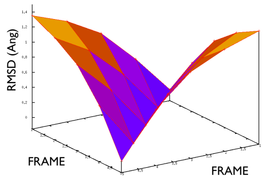
Hopefully the previous sections have allowed you to understand how PATH collective variables work and the sorts of problems they might be used to solve. If you have one of these problems to solve the next reasonable question to ask is: how to collect the set of reference frames that serve as the way markers on your PATH. Unfortunately, there is no single answer to this question. Different researchers have used different methods including using packages that morph one protein structure into another, using information from prior molecular dynamics or enhanced sampling calculations and even using PATH collective variables that change adaptively as the simulation progresses. Ultimately, you will need to find the best method for solving your particular problem. Having said that, however, there is some general guidance on setting up PATH collective variable and it is this that we will focus on in this section. The first thing that you will need to double check is the spacing between the frames in your PATH. Lets suppose that your PATH has \(N\) of these way markers upon it you will need to calculate is the \(N \times N\) matrix of distances between way markers. That is to say you will have to calculate the distance \(\vertX_j-X_i\vert\) between each pair of frames. The values of the distance in this matrix for a good PATH are shown in the figure below:
For contrast the values of the distances in this matrix for a bad PATH are shown in the figure below:
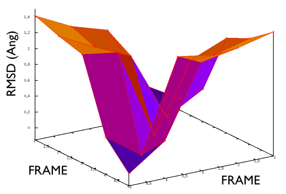
If the distance matrix looks like the second of the two figures shown above this is indicates that the frames in the PATH that have been chosen are not particularly effective. Lets suppose that we have a PATH with four way markers upon it. In order for the \(S(x)\) CV that was defined earlier to work well frame number 3 must be further from frame number 1 than frame number 2. Similarly frame number 4 must be still further from frame number 1 than frame number 3. This is what the gull wing shape in marvel-2-good-matrix-fig is telling us. The order of the frames in the rows and columns of the matrix is the same as the order that they are run through in the sums in the equation for \(S(X)\). The shape of the surface in this figure shows that the distance between frames \(i\) and \(j\) increases monotonically as the magnitude of the difference between \(i\) and \(j\) is increased, which is what is required.
A second important requirement of a good PATH is shown in the figure below:
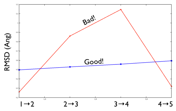
A good PATH has an approximately equal spacing between the neighboring frames along it. In other words, the distance between frame 1 and frame 2 is approximately equal to the distance between frame 2 and frame 3 as shown above. When this condition is satisfied a good criterion for selecting a suitable \(\lambda\) parameter to use is:
\[ \lambda=\frac{2.3 (N-1) }{\sum_{i=1}^{N-1} \vert X_i-X_{i+1} \vert } \]
If you have worked through all of this tutorial make sure that you have understood it by ensuring that you understand what the list of learning outcomes in section Learning Outcomes means and that you can use PLUMED to perform all these tasks. You might then want to read the original paper on the PATH collective variable method as well as a few other articles in which these coordinates have been used to analyze simulations and to accelerate sampling.
If you are interested in learning more about isocommittor surfaces and the transition state ensemble you should read up on the transition path sampling method.
 1.8.14