 |
|
|
| |
|
|
The aim of this tutorial is to introduce users to the PLUMED syntax. We will go through the preparation of input files to calculate and print simple collective variables on a pre-calculated trajectory. This tutorial has been prepared by Max Bonomi (adapting a lot of material from other tutorials) for the Master In Silico Drug Design, held at Universite' de Paris on November 25th, 2020.
Once this tutorial is completed, users will be able to:
In this and in the next tutorial, we will use two pieces of software: PLUMED version 2.6.2 and GROMACS version 2019.6. Both codes have already been installed on your machines and are ready to use. If you are attending the tutorial on Zoom, please have a look below at the section "Install GROMACS+PLUMED on your own machine with Conda".
PLUMED is a library that can be incorporated into many MD codes by adding a relatively simple and well documented interface. Once it is incorporated you can use PLUMED to perform a variety of different analyses on-the-fly and to bias the sampling in MD simulations. Additionally, PLUMED can be used as a standalone code for analyzing trajectories. If you are using the code in this way you can run the PLUMED executable by issuing the command:
plumed <instructions>
Let's start by getting a feel for the range of calculations that PLUMED can do. Issue the following command now:
plumed --help
The output of this command is a list of tasks that PLUMED can perform. Among these, there are commands that allow you to patch an MD code, postprocess metadynamics simulations, and build the manual. In this tutorial we will mostly use PLUMED to analyze trajectories. In order to do so, we will learn how to use the driver tool. Let's look at the options of PLUMED driver by issuing the following command:
plumed driver --help
As you can see we can do a number of things with PLUMED driver. For all of these options, however, we are going to need to write a PLUMED input file. The syntax of the PLUMED input file is the same that we will use later to run enhanced sampling simulations during a MD simulation, so all the things that you will learn now will be useful later when you will run PLUMED coupled to GROMACS.
GROMACS is a molecular dynamics package mainly designed for simulations of proteins, lipids, and nucleic acids. More info can be found here.
To be able to use GROMACS on your machine, you need to execute the following command line in your bash terminal:
source /opt/sdv/gromacs-2019.6/bin/GMXRC
You need to execute the command above in every new terminal window (shell) you open. Alternatively, you can add the line to the file .bashrc located in your home directory. After doing this, you can open a new shell and check that GROMACS is properly working by typing:
gmx mdrun -h
If you inspect the long output generated by this command, you will notice a -plumed option, which indicates that GROMACS has properly been compiled with PLUMED. Great, now you are ready to go!
In the eventuality in which you cannot find the software on your machine or you are working remotely, you can find a pre-compiled version of GROMACS 2018.8 patched with PLUMED version 2.6.2 on Conda. First, check if Conda is installed on your machine by typing: In case the command is not found, please follow the instructions below to install Conda in the directory Now you can open a new shell and create a separate environment for the ISDD tutorial using the following commands: Finally, you can install the pre-compiled version of GROMACS 2018.8 patched with PLUMED 2.6.2: and check your installation by typing: If you inspect the long output generated by this command, you will notice a Keep in mind that every time you open a new shell, in order to use PLUMED and GROMACS you need to activate the To learn more: Install GROMACS+PLUMED on your own machine with Conda
conda
/path/to/conda. You can choose it in your home so that you will have write permission to it.# on Linux:
wget -c https://repo.continuum.io/miniconda/Miniconda3-latest-Linux-x86_64.sh -O miniconda.sh
# on MacOS:
# wget -c https://repo.continuum.io/miniconda/Miniconda3-latest-MacOSX-x86_64.sh -O miniconda.sh
bash ./miniconda.sh -b -f -p /path/to/conda
# export PATH to find the Conda executable
export PATH="/path/to/conda/bin:$PATH"
# initialize bash shell
conda init bash
# create environment
conda create --name ISDD-tutorial
# activate environment
conda activate ISDD-tutorial
conda install -c plumed/label/munster -c conda-forge gromacs
gmx mdrun -h
-plumed option, which indicates that GROMACS has properly been compiled with PLUMED. Great, now you are ready to go!ISDD-tutorial Conda environment using the following command:conda activate ISDD-tutorial
The main goal of PLUMED is to compute collective variables (or CVs), which are complex descriptors of the system that can be used to describe the conformational change of a protein or a chemical reaction. This can be done either on-the-fly during a molecular dynamics simulations or a posteriori on a pre-calculated trajectory using PLUMED as a post-processing tool. In both cases one, you should create an input file with a specific PLUMED syntax. Have a look at the sample input file below:
# Compute distance between atoms 1 and 10.
# Atoms are ordered as in the trajectory files and their numbering starts from 1.
# The distance is called "d" for future reference.
d: DISTANCE ATOMS=1,10

# Compute the torsional angle between atoms 1, 10, 20, and 30.
# The angle is called "phi1" for future reference.
phi1: TORSION ATOMS=1,10,20,30

# The same CV defined above can be split into multiple lines
# The angle is called "phi2" for future reference.
TORSION ...
LABEL=phi2
ATOMS=1,10,20,30
...

# Print "d" on a file named "COLVAR1" every 10 steps.
PRINT ARG=d FILE=COLVAR1 STRIDE=10

# Print "phi1" and "phi2" on another file named "COLVAR2" every 100 steps.
PRINT ARG=phi1,phi2 FILE=COLVAR2 STRIDE=100
In the input file above, each line defines a so-called action. In this simple example, actions are used to compute a distance, a dihedral angle, or print some values on a file. Each action supports a number of keywords, whose value is specified. Action names are highlighted in green and, by clicking on them, you can go to the corresponding page in the manual that contains a detailed description of each keyword. Actions that support the keyword STRIDE are those that determine how frequently things are done. Notice that the default value for STRIDE is always 1. In the example above, omitting STRIDE keywords the corresponding COLVAR files would have been written for every frame of the analyzed trajectory. All the other actions in the example above, i.e. DISTANCE and TORSION, do not support the STRIDE keyword and are only calculated when requested. That is, d will be computed every 10 frames, and phi1 and phi2 every 100 frames.
Variables should be given a name (in the example above, d, phi1, and phi2), which is then used to refer to these variables in subsequent actions, such as the PRINT command. A lists of atoms should be provided as comma separated numbers, with no space.
You can find more information on the PLUMED syntax at Getting Started page of the manual. The complete documentation for all the supported collective variables can be found at the Collective Variables page.
By default the PLUMED inputs and outputs quantities in the following units:
If you want to change these units, you can do this using the UNITS keyword.
The TARBALL for this tutorial contains the following files:
GB1_native.pdb: a PDB file with the native structure of the GB1 protein.traj-whole.xtc: a trajectory in xtc format. GB1 has already been made whole by fixing discontinuities due to periodic boundary conditions.traj-broken.xtc: the same trajectory as it was originally produced by GROMACS. Here GB1 is broken by periodic boundary conditions.After dowloading the compressed archive to your local machine, you can unpack it using the following command:
tar xvzf master-ISDD-1.tar.gz
Once unpacked, all the files can be found in the master-ISDD-1 directory. To keep things clean, it is recommended to run each exercise in a separate sub-directory that you can create inside master-ISDD-1.
In this exercise, we will learn how to compute and print collective variables on a pre-calculated MD trajectory. To analyze the trajectories provided here, we will:
plumed.dat);Notice that you can also visualize trajectories with VMD (always a good idea!). For example, the trajectory traj-whole.xtc can be visualized with the command:
vmd GB1_native.pdb traj-whole.xtc
Let's now prepare a PLUMED input file to calculate:
GB1_native.pdb file to retrieve the list of indexes of the CA atoms;R_0 to 8.0 Angstrom (be careful with units!).Below you can find a sample plumed.dat file that you can use as a template. Whenever you see an highlighted FILL string, be careful because this is a string that you must replace.
# Compute gyration radius on CA atoms:
r: GYRATION ATOMS=__FILL__

# Compute number of contacts between CA atoms
co: COORDINATION GROUPA=__FILL__ R_0=__FILL__

# Print the two collective variables on COLVAR file every step
PRINT ARG=__FILL__ FILE=COLVAR STRIDE=__FILL__
Once your plumed.dat file is complete, you can run the PLUMED driver as follows:
> plumed driver --plumed plumed.dat --mf_xtc traj-broken.xtc
Scroll in your terminal to read the PLUMED log. As you can see, PLUMED gives a lot of feedback about the input that it is reading and the actions that it will execute. Please take your time to inspect the log file and check if PLUMED is actually doing what you intend to do.
The command above will create a COLVAR file like this one:
#! FIELDS time r co
 0.000000 2.458704 165.184127
 1.000000 2.341932 164.546604
 2.000000 2.404708 162.606975
 3.000000 2.454297 143.850122
 4.000000 2.569342 147.110408
 5.000000 2.304027 163.608703
Notice that the first line informs you about the content of each column.
In case you obtain different numbers, check your input, you might have made some mistake!
This file can then be visualized using gnuplot (for more info about this tool, look here):
gnuplot> p "COLVAR" u 1:2, "" u 1:3
Now, look at what happens if you run the exercise twice. The second time, PLUMED will back up the previously produced file so as not to overwrite it. You can also concatenate your files by using the action RESTART at the beginning of your input file.
Finally, let's try to use the same input file with traj-whole.xtc and examine the results. Did you find the same results as with the previous trajectory? Why?
PLUMED provides some shortcuts to select atoms with specific properties. To use this feature, you should specify the MOLINFO action along with a reference PDB file. This command is used to provide information on the molecules that are present in your system.
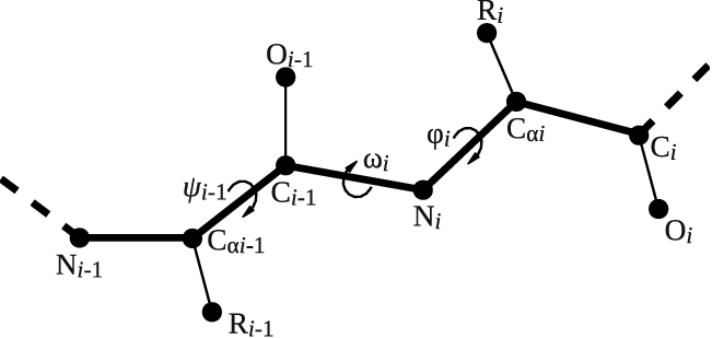
Let's try to use this functionality to calculate the backbone dihedral angle \( \phi \) (phi) of residue 2 of the GB1 protein. This CV is defined by the action TORSION and a set of 4 atoms. For residue i, the dihedral \( \phi \) is defined by these atoms: C(i-1),N(i),CA(i),C(i) (see Fig. master-ISDD-1-dih-fig).
After consulting the manual and inspecting GB1_native.pdb, let's define the dihedral angle \( \phi \) of residue 2 in two different ways:
t1).t2);# Activate MOLINFO functionalities MOLINFO STRUCTURE=__FILL__ # Define the dihedral phi of residue 2 as an explicit list of 4 atoms t1: TORSION ATOMS=__FILL__ # Define the same dihedral using MOLINFO shortcuts t2: TORSION ATOMS=__FILL__ # Print the two collective variables on COLVAR file every 10 steps PRINT ARG=__FILL__ FILE=COLVAR STRIDE=__FILL__
After completing the PLUMED input file above, let's use it to analyze the trajectory traj-whole.xtc using the driver tool:
> plumed driver --plumed plumed.dat --mf_xtc traj-whole.xtc
You can use gnuplot to visualize the trajectory of the two CVs calculated with the PLUMED input file above and written in the COLVAR file. If you executed this exercise correctly, these two trajectories should be identical.
Sometimes, when calculating a CV, you may not want to use the positions of a number of atoms directly. Instead you may want to define a virtual atom whose position is generated based on the positions of a collection of other atoms. For example you might want to use the center of mass (COM) or the geometric center (CENTER) of a group of atoms.
In this exercise, you will learn how to specify virtual atoms and later use them to define a CV. Let's start by having a look at the PLUMED input file below.
# Geometric center of first residue
first: CENTER ATOMS=1,2,3,4,5,6,7,8
# Geometric center of last residue
last: CENTER ATOMS=427-436

# Distance between centers of first and last residues, with PBCs
d1: DISTANCE ATOMS=first,last
# Distance between centers of first and last residues, without PBCs
d2: DISTANCE ATOMS=first,last NOPBC

# Print the two distances on COLVAR file every step
PRINT ARG=__FILL__ FILE=COLVAR STRIDE=__FILL__
The file above instructs PLUMED to:
first as the CENTER of atoms from 1 to 8;last as the CENTER of atoms from 427 to 436;first and last and saves it in d1;first and last and saves it in d2;d1 and d2 in the file COLVAR for every frame of the trajectory.Notice that in the input above we have used two different ways of writing the atoms used in the CENTER calculation:
ATOMS=1,2,3,4,5,6,7,8 is the explicit list of the atoms we need;ATOMS=427-436 is the range of atoms needed.Once you have prepared a PLUMED input file containing the above instructions, you can execute it on the trajectory traj-broken.xtc by making use of the following command:
plumed driver --mf_xtc traj-broken.xtc --plumed plumed.dat
Let's now analyze the output of the calculation by plotting the time series of the two CVs. Are they identical? What do you think is happening in those frames in which the two CVs are different?
You can repeat the same analysis on traj-whole.xtc and compare with the previous trajectory. Are the results identical?
In summary, in this tutorial you should have learned how to use PLUMED to:
 1.8.14