 |
|
|
| |
|
|
The primary aim of this Masterclass is to show you how you might use PLUMED in your work. We will see how to call PLUMED from a python notebook and discuss some strategies for selecting collective variables.
Once this Masterclass is completed, users will be able to:
Throughout this exercise, we use the atomistic simulation environment:
https://wiki.fysik.dtu.dk/ase/
and chemiscope:
Please look at the websites for these codes that are given above for more information.
For this Masterclass, you will need to set up the plumed and gromacs as you did for PLUMED Masterclass 21.5: Simulations with multiple replicas. You thus install plumed and gromacs using:
conda install --strict-channel-priority -c plumed/label/masterclass-mpi -c conda-forge plumed
conda install --strict-channel-priority -c plumed/label/masterclass-mpi -c conda-forge gromacs
You can install the other software you need using:
conda install -c conda-forge py-plumed Numpy pandas matplotlib notebook mdtraj mdanalysis git ase
Notice that you need a package called ase (the atomic simulation environment) for these exercises and the other packages you have been using. You also need to install chemiscope, which you can do by using the following command:
pip install chemiscope
The data needed to complete this Masterclass can be found on GitHub. You can clone this repository locally on your machine using the following command:
git clone https://github.com/plumed/masterclass-21-6.git
I recommend that you run each exercise in a separate sub-directory (i.e. Exercise-1, Exercise-2, ...), which you can create inside the root directory masterclass-21-6. Organizing your data this way will help you to keep things clean.
I like working with Python notebooks. Using notebooks allows me to keep the codes that I am working on close to the explanations of how these codes work. I can also make all my figures within a notebook. By using notebooks, I can thus have a single file that contains:
In previous masterclasses we have run plumed driver through bash from within a notebook by using commands like the one shown below:
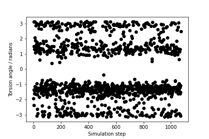
We have then read in the colvar file produced and analyzed it from within the notebook. We can avoid using plumed driver and can call plumed directly from python using the python interface. The code below, for instance, generates the plot underneath the code. The code reads in the trajectory from the file traj.pdb that you obtained from the GitHub repository. The plot then shows how the \(\phi\) angle on the second residue of the protein changes with time.
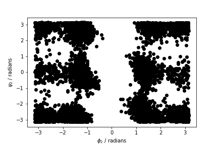
Your task in this first exercise is to modify the code above and to produce a figure similar to the one shown below. This figure shows all the values of the \(\phi\) and \(\psi\) angles in the second residue of the protein during the simulation.
Plots showing the trajectory in CV space similar to those you generated at the end of the previous exercise are helpful. What would be more useful, however, is some way of understanding the relationship between the positions in CV space and the structures of the various atoms. In other words, what we would like is something like this:
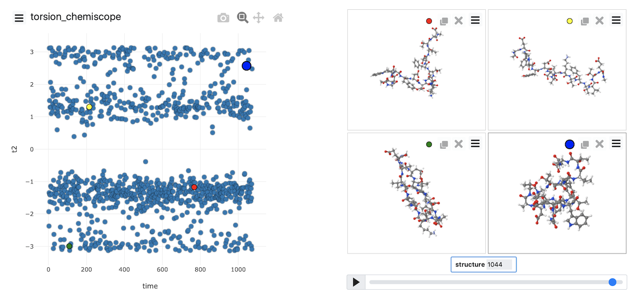
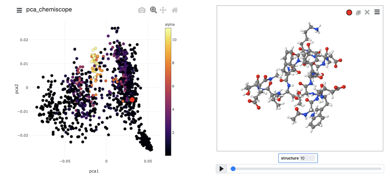
You can see the frame in the trajectory that each point in the plot corresponds to from the above figure. The snapshots on the right correspond to the structures the system had at the points highlighted in red, yellow, green and blue respectively in the plot on the left.
The figure above was generated using chemiscope.
This server allows you to generate and interact with plots like the one shown above. Your task in this exercise is to generate your own chemiscope representation of the data in traj.pdb. To create a chemiscope representation of the \(\phi\) angles that we generated using the first python script from the previous exercise, you would add the following python code:
You would then upload the torsion_chemiscope.json.gz file that is generated by this script at https://chemiscope.org.
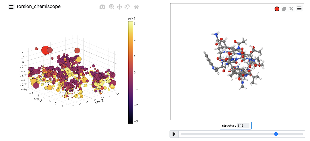
See if you can generate your own chemiscope representation of the data in traj.pdb. I would recommend calculating and uploading a chemiscope representation of all the protein's torsional angles.
At the very least, you need to do at least two backbone torsional angles. However, if you do more than two torsions, you can generate a plot like the one shown below.
Chemiscope comes into its own when you are working with a machine learning algorithm. These algorithms can (in theory) learn the collective variables you need to use from the trajectory data. To make sense of the coordinates that have been learned, you have to carefully visualize where structures are projected in the low dimensional space. You can use chemiscope to complete this process of visualizing the representation the computer has found for you. In this next set of exercises, we will apply various dimensionality reduction algorithms to the data contained in the file traj.pdb. If you visualize the contents of that file using VMD, you will see that this file contains a short protein trajectory. You are perhaps unsure what CV to analyze this data and thus want to see if you can shed any light on the contents of the trajectory by using machine learning.
Typically, PLUMED analyses one set of atomic coordinates at a time. To run a machine learning algorithm, however, you need to gather information on multiple configurations. Therefore, the first thing you need to learn to use these algorithms is how to store configurations for later analysis with a machine learning algorithm. The following input illustrates how to complete this task using PLUMED.
# This reads in the template pdb file and thus allows us to use the @nonhydrogens # special group later in the input MOLINFOSTRUCTURE=__FILL__compulsory keyword a file in pdb format containing a reference structure.MOLTYPE=protein # This stores the positions of all the nonhydrogen atoms for later analysis cc: COLLECT_FRAMEScompulsory keyword ( default=protein ) what kind of molecule is contained in the pdb file - usually not needed since protein/RNA/DNA are compatible__FILL__=@nonhydrogens # This should output the atomic positions for the frames that were collected to a pdb file called traj.pdb OUTPUT_ANALYSIS_DATA_TO_PDBcould not find this keywordUSE_OUTPUT_DATA_FROM=__FILL__use the output of the analysis performed by this object as input to your new analysis objectFILE=traj.pdbcompulsory keyword the name of the file to output to
Copy the input above into a plumed file and fill in the blanks. You should then be able to run the command using:
Then, once all the blanks are filled in, run the command using:
plumed driver --mf_pdb traj.pdb
You can also store the values of collective variables for later analysis with these algorithms. Modify the input above so that all Thirty backbone dihedral angles in the protein are stored, and output using OUTPUT_ANALYSIS_DATA_TO_COLVAR and rerun the calculation.
For more information on the dimensionality reduction algorithms that we are using in this section see:
https://arxiv.org/abs/1907.04170
Having learned how to store data for later analysis with a dimensionality reduction algorithm, lets now apply principal component analysis (PCA) upon our stored data. In principle component analysis, low dimensional projections for our trajectory are constructed by:
To perform PCA using PLUMED, we are going to use the following input with the blanks filled in:
# This reads in the template pdb file and thus allows us to use the @nonhydrogens # special group later in the input MOLINFOSTRUCTURE=__FILL__compulsory keyword a file in pdb format containing a reference structure.MOLTYPE=protein # This stores the positions of all the nonhydrogen atoms for later analysis cc: COLLECT_FRAMEScompulsory keyword ( default=protein ) what kind of molecule is contained in the pdb file - usually not needed since protein/RNA/DNA are compatible__FILL__=@nonhydrogens # This diagonalizes the covariance matrix pca: PCAcould not find this keywordUSE_OUTPUT_DATA_FROM=__FILL__use the output of the analysis performed by this object as input to your new analysis objectMETRIC=OPTIMALcompulsory keyword ( default=EUCLIDEAN ) the method that you are going to use to measure the distances between pointsNLOW_DIM=2 # This projects each of the trajectory frames onto the low dimensional space that was # identified by the PCA command dat: PROJECT_ALL_ANALYSIS_DATAcompulsory keyword number of low-dimensional coordinates requiredUSE_OUTPUT_DATA_FROM=__FILL__use the output of the analysis performed by this object as input to your new analysis objectPROJECTION=__FILL__ # This should output the PCA projections of all the coordinates OUTPUT_ANALYSIS_DATA_TO_COLVARcompulsory keyword the projection that you wish to generate out-of-sample projections withUSE_OUTPUT_DATA_FROM=__FILL__use the output of the analysis performed by this object as input to your new analysis objectARG=dat.*the input for this action is the scalar output from one or more other actions.FILE=pca_data # These next three commands calculate the secondary structure variables. These # variables measure how much of the structure resembles an alpha helix, an antiparallel beta-sheet # and a parallel beta-sheet. Configurations that have different secondary structures should be projected # in different parts of the low dimensional space. alpha: ALPHARMSDcompulsory keyword the name of the file to output toRESIDUES=all abeta: ANTIBETARMSDthis command is used to specify the set of residues that could conceivably form part of the secondary structure.RESIDUES=allthis command is used to specify the set of residues that could conceivably form part of the secondary structure.STRANDS_CUTOFF=1.0 pbeta: PARABETARMSDIf in a segment of protein the two strands are further apart then the calculation of the actual RMSD is skipped as the structure is very far from being beta-sheet like.RESIDUES=allthis command is used to specify the set of residues that could conceivably form part of the secondary structure.STRANDS_CUTOFF=1.0 # These commands collect and output the secondary structure variables so that we can use this information to # determine how good our projection of the trajectory data is. cc2: COLLECT_FRAMESIf in a segment of protein the two strands are further apart then the calculation of the actual RMSD is skipped as the structure is very far from being beta-sheet like.ARG=alpha,abeta,pbeta OUTPUT_ANALYSIS_DATA_TO_COLVARthe input for this action is the scalar output from one or more other actions.USE_OUTPUT_DATA_FROM=cc2use the output of the analysis performed by this object as input to your new analysis objectARG=cc2.*the input for this action is the scalar output from one or more other actions.FILE=secondary_structure_datacompulsory keyword the name of the file to output to
To generate the projection, you run the command:
plumed driver --mf_pdb traj.pdb
You can generate a projection of the data above using chemiscope by using the following script:
When the output from this set of commands is loaded into chemiscope, we can construct figures like the one shown below. On the axes here, we have plotted the PCA coordinates. The points are then coloured according to the alpha-helical content.
See if you can use PLUMED and chemiscope to generate a figure similar to the one above. Try to experiment with the way the points are coloured. Look at the beta-sheet content as well.
In the previous section, we performed PCA on the atomic positions directly. In the section before last, however, we also saw how we could store high-dimensional vectors of collective variables and then use them as input to a dimensionality reduction algorithm. Therefore, we might legitimately ask if we can do PCA using these high-dimensional vectors as input rather than atomic positions. The answer to this question is yes as long as the CV is not periodic. If any of our CVs are not periodic, we cannot analyze them using the PCA action. We can, however, formulate the PCA algorithm differently. In this alternative formulation, which is known as classical multidimensional scaling (MDS), we do the following:
This method is used less often than PCA as the matrix that we have to diagonalize here in the third step can be considerably larger than the matrix that we have to diagonalize when we perform PCA.
To avoid this expensive diagonalization step, we often select a subset of so-called landmark points on which to run the algorithm directly. Projections for the remaining points are then found by using a so-called out-of-sample procedure. This is what has been done in the following input:
THIScommandcould not find this keywordreadscould not find this keywordincould not find this keywordthecould not find this keywordtemplatecould not find this keywordpdbcould not find this keywordfilecould not find this keywordandcould not find this keywordthuscould not find this keywordallowscould not find this keyworduscould not find this keywordtocould not find this keywordusecould not find this keywordthecould not find this keyword@nonhydrogens# group later in the input MOLINFOcould not find this keywordSTRUCTURE=beta-hairpin.pdbcompulsory keyword a file in pdb format containing a reference structure.MOLTYPE=protein # This stores the positions of all the nonhydrogen atoms for later analysis cc: COLLECT_FRAMEScompulsory keyword ( default=protein ) what kind of molecule is contained in the pdb file - usually not needed since protein/RNA/DNA are compatibleATOMS=@nonhydrogens # The following commands compute all the Ramachandran angles of the protein for you r2-phi: TORSIONthe atoms whose positions we are tracking for the purpose of analyzing the dataATOMS=@phi-2 r2-psi: TORSIONthe four atoms involved in the torsional angleATOMS=@psi-2 r3-phi: TORSIONthe four atoms involved in the torsional angleATOMS=@phi-3 r3-psi: TORSIONthe four atoms involved in the torsional angleATOMS=@psi-3 r4-phi: TORSION __FILL__ r4-psi: TORSION __FILL__ r5-phi: TORSION __FILL__ r5-psi: TORSION __FILL__ r6-phi: TORSION __FILL__ r6-psi: TORSION __FILL__ r7-phi: TORSION __FILL__ r7-psi: TORSION __FILL__ r8-phi: TORSION __FILL__ r8-psi: TORSION __FILL__ r9-phi: TORSION __FILL__ r9-psi: TORSION __FILL__ r10-phi: TORSION __FILL__ r10-psi: TORSION __FILL__ r11-phi: TORSION __FILL__ r11-psi: TORSION __FILL__ r12-phi: TORSION __FILL__ r12-psi: TORSION __FILL__ r13-phi: TORSION __FILL__ r13-psi: TORSION __FILL__ r14-phi: TORSION __FILL__ r14-psi: TORSION __FILL__ r15-phi: TORSION __FILL__ r15-psi: TORSION __FILL__ r16-phi: TORSION __FILL__ r16-psi: TORSION __FILL__ # This command stores all the Ramachandran angles that were computed angles: COLLECT_FRAMESthe four atoms involved in the torsional angle__FILL__=r2-phi,r2-psi,r3-phi,r3-psi,r4-phi,r4-psi,r5-phi,r5-psi,r6-phi,r6-psi,r7-phi,r7-psi,r8-phi,r8-psi,r9-phi,r9-psi,r10-phi,r10-psi,r11-phi,r11-psi,r12-phi,r12-psi,r13-phi,r13-psi,r14-phi,r14-psi,r15-phi,r15-psi,r16-phi,r16-psi # Lets now compute the matrix of distances between the frames in the space of the Ramachandran angles distmat: EUCLIDEAN_DISSIMILARITIEScould not find this keywordUSE_OUTPUT_DATA_FROM=__FILL__use the output of the analysis performed by this object as input to your new analysis objectMETRIC=EUCLIDEAN # Now select 500 landmark points to analyze fps: LANDMARK_SELECT_FPScompulsory keyword ( default=EUCLIDEAN ) the method that you are going to use to measure the distances between pointsUSE_OUTPUT_DATA_FROM=__FILL__use the output of the analysis performed by this object as input to your new analysis objectNLANDMARKS=500 # Run MDS on the landmarks mds: CLASSICAL_MDScompulsory keyword the number of landmarks that you would like to select__FILL__=fpscould not find this keywordNLOW_DIM=2 # Project the remaining trajectory data osample: PROJECT_ALL_ANALYSIS_DATAcompulsory keyword number of low-dimensional coordinates requiredUSE_OUTPUT_DATA_FROM=__FILL__use the output of the analysis performed by this object as input to your new analysis objectPROJECTION=__FILL__ # This command outputs all the projections of all the points in the low dimensional space OUTPUT_ANALYSIS_DATA_TO_COLVARcompulsory keyword the projection that you wish to generate out-of-sample projections withUSE_OUTPUT_DATA_FROM=__FILL__use the output of the analysis performed by this object as input to your new analysis objectARG=osample.*the input for this action is the scalar output from one or more other actions.FILE=mds_data # These next three commands calculate the secondary structure variables. These # variables measure how much of the structure resembles an alpha helix, an antiparallel beta-sheet # and a parallel beta-sheet. Configurations that have different secondary structures should be projected # in different parts of the low dimensional space. alpha: ALPHARMSDcompulsory keyword the name of the file to output toRESIDUES=all abeta: ANTIBETARMSDthis command is used to specify the set of residues that could conceivably form part of the secondary structure.RESIDUES=allthis command is used to specify the set of residues that could conceivably form part of the secondary structure.STRANDS_CUTOFF=1.0 pbeta: PARABETARMSDIf in a segment of protein the two strands are further apart then the calculation of the actual RMSD is skipped as the structure is very far from being beta-sheet like.RESIDUES=allthis command is used to specify the set of residues that could conceivably form part of the secondary structure.STRANDS_CUTOFF=1.0 # These commands collect and output the secondary structure variables so that we can use this information to # determine how good our projection of the trajectory data is. cc2: COLLECT_FRAMESIf in a segment of protein the two strands are further apart then the calculation of the actual RMSD is skipped as the structure is very far from being beta-sheet like.ARG=alpha,abeta,pbeta OUTPUT_ANALYSIS_DATA_TO_COLVARthe input for this action is the scalar output from one or more other actions.USE_OUTPUT_DATA_FROM=cc2use the output of the analysis performed by this object as input to your new analysis objectARG=cc2.*the input for this action is the scalar output from one or more other actions.FILE=secondary_structure_datacompulsory keyword the name of the file to output to
This input collects all the torsional angles for the configurations in the trajectory. Then, at the end of the calculation, the matrix of distances between these points is computed, and a set of landmark points is selected using a method known as farthest point sampling. A matrix that contains only those distances between the landmarks is then constructed and diagonalized by the CLASSICAL_MDS action so that projections of the landmarks can be built. The final step is then to project the remainder of the trajectory using the PROJECT_ALL_ANALYSIS_DATA action. Try to fill in the blanks in the input above and run this calculation now using the command:
plumed driver --mf_pdb traj.pdb
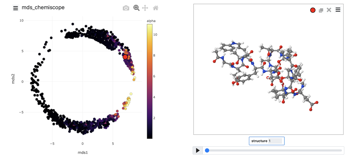
Once the calculation has completed, you can, once again, visualize the data using chemiscope by using a suitably modified version of the script from the previous exercise. The image below shows the MDS coordinates coloured according to the alpha-helical content.
Try to generate an image that looks like this one yourself by completing the input above and then using what you learned about generating chemiscope representations in the previous exercise.
The two algorithms (PCA and MDS) that we have looked at thus far are linear dimensionality reduction algorithms. In addition to these, there are a whole class of non-linear dimensionality reduction reduction algorithms which work by transforming the matrix of dissimilarities between configurations, calculating geodesic rather than Euclidean distances between configurations or by changing the form of the loss function that is optimized. In this final exercise, we will use an algorithm that uses the last of these three strategies to construct a non-linear projection. The algorithm is known as sketch-map and input for sketch-map is provided below:
# This reads in the template pdb file and thus allows us to use the @nonhydrogens # special group later in the input MOLINFOSTRUCTURE=__FILL__compulsory keyword a file in pdb format containing a reference structure.MOLTYPE=protein # This stores the positions of all the nonhydrogen atoms for later analysis cc: COLLECT_FRAMEScompulsory keyword ( default=protein ) what kind of molecule is contained in the pdb file - usually not needed since protein/RNA/DNA are compatible__FILL__=@nonhydrogens # This should output the atomic positions for the frames that were collected and analyzed using MDS OUTPUT_ANALYSIS_DATA_TO_PDBcould not find this keywordUSE_OUTPUT_DATA_FROM=__FILL__use the output of the analysis performed by this object as input to your new analysis objectFILE=traj.pdb # The following commands compute all the Ramachandran angles of the protein for you r2-phi: TORSIONcompulsory keyword the name of the file to output toATOMS=@phi-2 r2-psi: TORSIONthe four atoms involved in the torsional angleATOMS=@psi-2 r3-phi: TORSIONthe four atoms involved in the torsional angleATOMS=@phi-3 r3-psi: TORSIONthe four atoms involved in the torsional angleATOMS=@psi-3 r4-phi: TORSION __FILL__ r4-psi: TORSION __FILL__ r5-phi: TORSION __FILL__ r5-psi: TORSION __FILL__ r6-phi: TORSION __FILL__ r6-psi: TORSION __FILL__ r7-phi: TORSION __FILL__ r7-psi: TORSION __FILL__ r8-phi: TORSION __FILL__ r8-psi: TORSION __FILL__ r9-phi: TORSION __FILL__ r9-psi: TORSION __FILL__ r10-phi: TORSION __FILL__ r10-psi: TORSION __FILL__ r11-phi: TORSION __FILL__ r11-psi: TORSION __FILL__ r12-phi: TORSION __FILL__ r12-psi: TORSION __FILL__ r13-phi: TORSION __FILL__ r13-psi: TORSION __FILL__ r14-phi: TORSION __FILL__ r14-psi: TORSION __FILL__ r15-phi: TORSION __FILL__ r15-psi: TORSION __FILL__ r16-phi: TORSION __FILL__ r16-psi: TORSION __FILL__ # This command stores all the Ramachandran angles that were computed angles: COLLECT_FRAMESthe four atoms involved in the torsional angle__FILL__=r2-phi,r2-psi,r3-phi,r3-psi,r4-phi,r4-psi,r5-phi,r5-psi,r6-phi,r6-psi,r7-phi,r7-psi,r8-phi,r8-psi,r9-phi,r9-psi,r10-phi,r10-psi,r11-phi,r11-psi,r12-phi,r12-psi,r13-phi,r13-psi,r14-phi,r14-psi,r15-phi,r15-psi,r16-phi,r16-psi # Lets now compute the matrix of distances between the frames in the space of the Ramachandran angles distmat: EUCLIDEAN_DISSIMILARITIEScould not find this keywordUSE_OUTPUT_DATA_FROM=__FILL__use the output of the analysis performed by this object as input to your new analysis objectMETRIC=EUCLIDEAN # Now select 500 landmark points to analyze fps: LANDMARK_SELECT_FPScompulsory keyword ( default=EUCLIDEAN ) the method that you are going to use to measure the distances between pointsUSE_OUTPUT_DATA_FROM=__FILL__use the output of the analysis performed by this object as input to your new analysis objectNLANDMARKS=500 # Run sketch-map on the landmarks smap: SKETCH_MAPcompulsory keyword the number of landmarks that you would like to select__FILL__=fpscould not find this keywordNLOW_DIM=2compulsory keyword the dimension of the low dimensional space in which the projections will be constructedHIGH_DIM_FUNCTION={SMAP R_0=6 A=8 B=2}compulsory keyword the parameters of the switching function in the high dimensional spaceLOW_DIM_FUNCTION={SMAP R_0=6 A=2 B=2}compulsory keyword the parameters of the switching function in the low dimensional spaceCGTOL=1E-3compulsory keyword ( default=1E-6 ) the tolerance for the conjugate gradient minimizationCGRID_SIZE=20compulsory keyword ( default=10 ) number of points to use in each grid directionFGRID_SIZE=200compulsory keyword ( default=0 ) interpolate the grid onto this number of points -- only works in 2DANNEAL_STEPS=0 # Project the remaining trajectory data osample: PROJECT_ALL_ANALYSIS_DATAcompulsory keyword ( default=10 ) the number of steps of annealing to doUSE_OUTPUT_DATA_FROM=__FILL__use the output of the analysis performed by this object as input to your new analysis objectPROJECTION=__FILL__ # This command outputs all the projections of all the points in the low dimensional space OUTPUT_ANALYSIS_DATA_TO_COLVARcompulsory keyword the projection that you wish to generate out-of-sample projections withUSE_OUTPUT_DATA_FROM=__FILL__use the output of the analysis performed by this object as input to your new analysis objectARG=osample.*the input for this action is the scalar output from one or more other actions.FILE=smap_data # These next three commands calculate the secondary structure variables. These # variables measure how much of the structure resembles an alpha helix, an antiparallel beta-sheet # and a parallel beta-sheet. Configurations that have different secondary structures should be projected # in different parts of the low dimensional space. alpha: ALPHARMSDcompulsory keyword the name of the file to output toRESIDUES=all abeta: ANTIBETARMSDthis command is used to specify the set of residues that could conceivably form part of the secondary structure.RESIDUES=allthis command is used to specify the set of residues that could conceivably form part of the secondary structure.STRANDS_CUTOFF=1.0 pbeta: PARABETARMSDIf in a segment of protein the two strands are further apart then the calculation of the actual RMSD is skipped as the structure is very far from being beta-sheet like.RESIDUES=allthis command is used to specify the set of residues that could conceivably form part of the secondary structure.STRANDS_CUTOFF=1.0 # These commands collect and output the secondary structure variables so that we can use this information to # determine how good our projection of the trajectory data is. cc2: COLLECT_FRAMESIf in a segment of protein the two strands are further apart then the calculation of the actual RMSD is skipped as the structure is very far from being beta-sheet like.ARG=alpha,abeta,pbeta OUTPUT_ANALYSIS_DATA_TO_COLVARthe input for this action is the scalar output from one or more other actions.USE_OUTPUT_DATA_FROM=cc2use the output of the analysis performed by this object as input to your new analysis objectARG=cc2.*the input for this action is the scalar output from one or more other actions.FILE=secondary_structure_datacompulsory keyword the name of the file to output to
This input collects all the torsional angles for the configurations in the trajectory. Then, at the end of the calculation, the matrix of distances between these points is computed, and a set of landmark points is selected using a method known as farthest point sampling. A matrix that contains only those distances between the landmarks is then constructed and diagonalized by the CLASSICAL_MDS action, and this set of projections is used as the initial configuration for the various minimization algorithms that are then used to optimize the sketch-map stress function. As in the previous exercise, once the projections of the landmarks are found, the projections for the remainder of the points in the trajectory are found by using the PROJECT_ALL_ANALYSIS_DATA action. Try to fill in the blanks in the input above and run this calculation now using the command:
plumed driver --mf_pdb traj.pdb
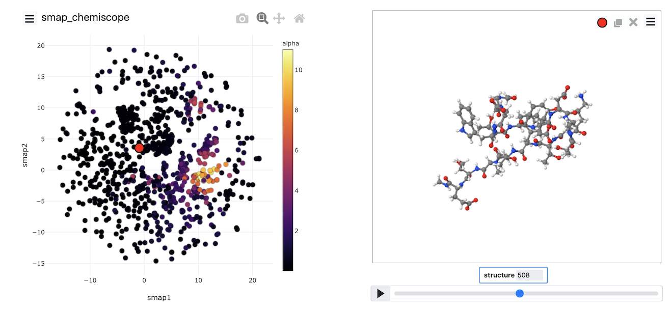
Once the calculation has completed, you can, once again, visualize the data generated using chemiscope by using the scripts from earlier exercises. My projection is shown in the figure below. Points are, once again, coloured following the alpha-helical content of the corresponding structure.
Try to see if you can reproduce an image that looks like the one above
This exercise has shown you that running dimensionality reduction algorithms using PLUMED involves the following stages:
There are multiple choices to be made in each of the various stages described above. For example, you can change the particular sort of data this is collected from the trajectory. There are multiple different ways to select landmarks. You can use the distances directly, or you can transform them. You can use various loss functions and optimize the loss function using a variety of different algorithms. When you tackle your own research problems using these methods, you can experiment with the various choices that can be made.
Generating a low-dimensional representation using these algorithms is not enough to publish a paper. We want to get some physical understanding from our simulation. Gaining this understanding is the hard part.
In many papers in this area, you will hear people talk about the distinction between collective variables and the reaction coordinate. The distinction these authors are trying emphasize when they use this language is between a descriptor that takes different values for the various important basins in the energy landscape (the collective variable) and the actual pathway the reaction proceeds along (the reaction coordinate). Furthermore, the authors of such papers will often argue that the reaction coordinate is simply some linear/non-linear combination of collective variables. In this exercise, we will study alanine dipeptide with path collective variables to show you one way of thinking about this distinction between collective variables and reaction coordinates.
By studying a system that is this simple, you will also hopefully come to understand how we can interpret the coordinates that we extract using the dimensionality reduction algorithms that were discussed in the previous exercise.
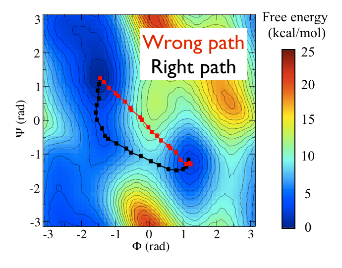
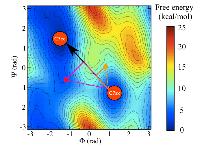
To remind you, the free energy surface as a function of the \(\phi\) and \(\psi\) angles for alanine dipeptide is shown below:

In other masterclasses, we have discussed how there are two critical states in the above energy landscape. These states are labelled C7eq and C7ax above.
The two Ramachandran angles plotted on the x and y axes of the free energy surface above are examples of what we have called collective variables. Both of these angles can be used to distinguish between C7eq and C7ax configurations. The reaction coordinate is the path that the system actually takes as it moves from the C7ax to the C7eq configuration. Based on the shape of the free energy surface, we might suppose that this reaction coordinate looks something like the black line shown below:
The file called alanine-transformation.pdb that you can find in the data directory of the GitHub repository contains a series of configurations that lie close to the transition path that is illustrated in black in the figure above. Below are plots that show how \(\phi\) and \(\psi\) change as the system moves along this path. Try to see if you can use what you have learned in previous masterclasses to reproduce the figure above before continuing.
We know what structures correspond to the various stable states of our system. We might, therefore, be tempted to ask ourselves if we can not just use the RMSD distance from a structure as the reaction coordinate. This approach will work if there is a single important configuration in the energy landscape. We could use the RMSD distance from this lowest energy structure as a CV to extract this configuration's free energy relative to everything else. How well does this work if we have two distinct states, though, as we have for alanine dipeptide? To investigate this question, fill in the PLUMED input below that calculates the RMSD distances from the C7ax and C7eq configurations:
c7ax: RMSD__FILL__=../data/C7ax.pdbcould not find this keywordTYPE=__FILL__ c7eq: RMSDcompulsory keyword ( default=SIMPLE ) the manner in which RMSD alignment is performed.__FILL__=../data/C7eq.pdbcould not find this keywordTYPE=__FILL__ PRINTcompulsory keyword ( default=SIMPLE ) the manner in which RMSD alignment is performed.ARG=c7ax,c7eqthe input for this action is the scalar output from one or more other actions.FILE=colvarthe name of the file on which to output these quantitiesSTRIDE=100'''compulsory keyword ( default=1 ) the frequency with which the quantities of interest should be output
You can run an MD simulation to monitor these distances using the python script below.
I ran simulations at 300K and 1000K using the above script. When the simulations completed, I was able to construct the figures below:
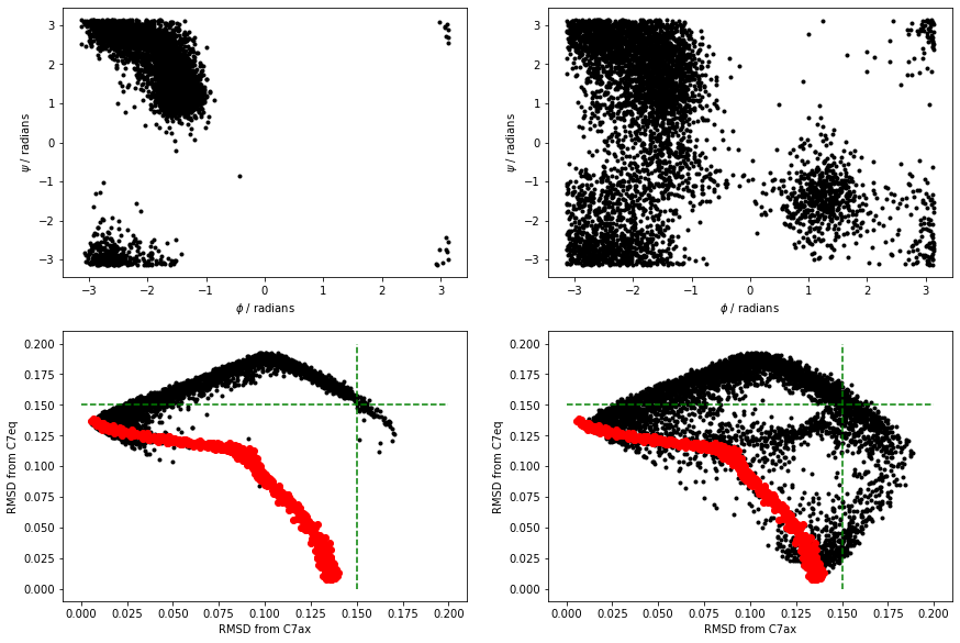
The black points above are the RMSD values for the trajectories. I have also shown the RMSD values for the frames in alanine-transformation in red. Notice that all the configurations explored in the MD are very distant from the C7ax and C7eq states. Try now to reproduce the above figure yourself.
You can see that at 300K, the simulation we ran did not visit the C7eq state. Furthermore, you can also clearly see this from the projections of the trajectories on the RMSD distances from these two configurations. Notice in these figures, however, that the distances from these two reference configurations were often considerably larger than the distance between these reference configurations and the configurations on the reference path in alanine-transformation.pdb.
Instead of calculating two distances, we might ask ourselves if the linear combination of \(\phi\) and \(\psi\) that is illustrated in the figure below:
gives a better description for the transition. We can define this CV as follows:
\[ s = \frac{(\phi_2 - \phi_1).(\phi_3 - \phi_1) + (\psi_2 - \psi_1).(\psi_3 - \psi_1)}{ \sqrt{(\phi_2 - \phi_1)^2 + (\psi_2 - \psi_1)^2} } \]
In this expression \((\phi_1,\psi_1)\) are the Ramachandran angles in the \(C_7eq\) configuration and \((\phi_2,\psi_2)\) are the Ramachandran angles in the \(C_7ax\). \((\phi_3,\psi_3)\) is the instantaneous configuration. You should thus be able to see that we have arrived at the above expression by using our knowledge of the dot product between two vectors.
See if you can write an input to re-analyse the data in alanine-transformation.pdb and the MD simulations from the previous section using this CV.
You should be able to get plots of the value of this CV as a function of step number that looks like the ones shown below:
I implemented this CV using a combination of TORSION and COMBINE. I also ignored the fact that the torsions are periodic variables when calculating the linear combination.
You can't use the sort of linear algebra above with periodic variables, but it is OK for these illustrative purposes.
Notice that the first frame in alanine-transformation.pdb has the molecule in the \(C_7ax\) configuration. The last frame has the molecule in the \(C_7eq\) state.
Figure masterclass-21-6-pca-figure showed how we can construct a new collective variables by taking a linear combination of two other variables. This idea can be extended to higher dimensions, however. As long as we can find the vector that connectes the \(C_7eq\) and \(C_7ax\) states we can project our current coordinates on that particular vector. We can even define this vector in the space of the coordinates of the atoms. In other words, if the 3 \(N\) coordinate of atomic positions is \(\mathbf{x}^{(1)}\) for the \(C_7eq\) configuration and \(\mathbf{x}^{(2)}\) for the \(C_7ax\) configuration and if the instantaneous configuration of the atoms is \(\mathbf{x}^{(3)}\) we can use the following as a CV:
\[ s = \frac{\sum_{i=1}^{3N} (x^{(2)}_i - x^{(1)}_i ) (x^{(3)}_i - x^{(1)}_i )}{ \sqrt{\sum_{i=1}^{3N} (x^{(2)}_i - x^{(1)}_i )^2} } \]
as long as rotational and translational movement is removed before calculating the two displacement vectors above.
We can also get some sense of how far the system has moved from this vector by computing:
\[ z = \sqrt{ \sum_{i=1}^{3N} (x^{(3)}_i - x^{(1)}_i)^2 - s^2 } \]
which follows by applying Pythagoras theorem.
You can calculate this collective variable using PLUMED by using the input below:
p: PCAVARS __FILL__=pca-reference.pdb __FILL__=OPTIMAL
PRINT ARG=p.* FILE=colvar
Use this input to re-analyse the data in alanine-transformation.pdb and your MD simulations before continuing. The figure below shows the results that I obtained by analyzing the data using the PCAVARS command above.
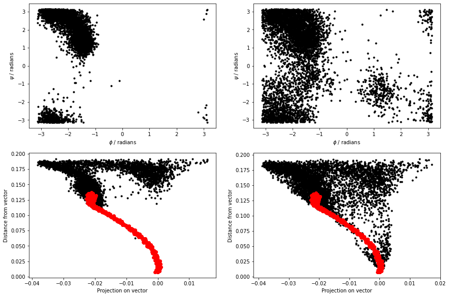
The figure above shows that this coordinate is good. We move quite far from this initial vector when we move to the C7ax state, however.
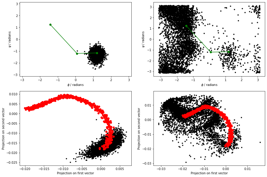
Instead of using a single PCA variable and calculating the projection on the vector connecting these two points, we can instead use the projection of the instantaneous coordinates in the plane that contains three reference configurations. You can calculate these collective variables using PLUMED by using the input below:
p: PCAVARS __FILL__=pca2-reference.pdb __FILL__=OPTIMAL
PRINT ARG=p.* FILE=colvar
Notice that there are now three structures within pca2-reference.pdb, and thus two vectors are defined. Use this input to re-analyse the data in alanine-transformation.pdb and your MD simulations before continuing.
The figure below shows the results that I obtained by analyzing the data using the PCAVARS command above.
Instead of using the projection on more than one vector, we can extend the ideas in the previous section and use curvilinear paths rather than linear paths. This trick is what is done with the PATH CVs that are illustrated in the figure below:
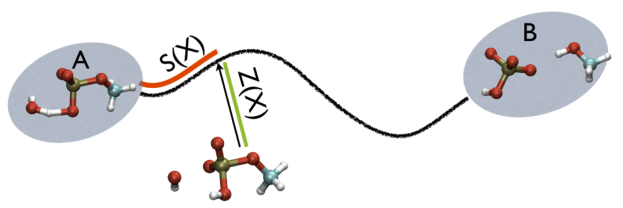
As you can see, there are two path collective variables, \(S(X)\) measures your position on a path and is calculated using:
\[ S(X)=\frac{\sum_{i=1}^{N} i\ \exp^{-\lambda \vert X-X_i \vert }}{ \sum_{i=1}^{N} \exp^{-\lambda \vert X-X_i \vert } } \]
\(Z(x)\), meanwhile, measures the distance from the path using:
\[ Z(X) = - \frac{1}{\lambda} \ln\left[ \sum_{i=1}^{N} \exp^{-\lambda \vert X-X_i \vert } \right] \]
We can calculate these CVs using a filled-in version of the input that is shown below:
path: PATH __FILL__=../data/alanine-path.pdb TYPE=__FILL__ LAMBDA=15100.
PRINT ARG=* FILE=colvar
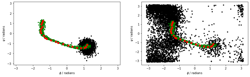
The figure below shows the \(\phi\) and \(\psi\) angles for the configurations that define the path as red dots. Meanwhile, the black dots are the \(\phi\) and \(\psi\) angles that are visited during a high temperature, unbiased MD trajectory. The green dots are then the configurations in alanine-transformation.pdb You can clearly see that the red dots lie along the transition path that connects the C7eq and C7ax configurations and that the green dots follow this pathway:
When we calculate the path collective variables for the black and red data points in the above figure, we get the result shown on the right. The panel on the left shows the output from a 300 K simulation during which the C7eq configuration was not visited:
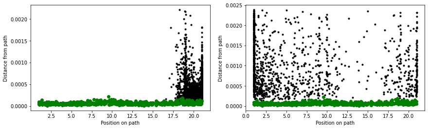
You can see that the majority of configurations have very small z values. It would thus seem that we have identified our reaction coordinate. We can use the S-path coordinate to tell us where we are on the transition pathway between the two states. Furthermore, in defining this coordinate, we have used the positions of all the heavy atoms in the protein.
Notice that when we talk about the reaction coordinate, we are not talking about a single set of configurations that connect the two states. The previous sections have shown that there are always multiple pathways that connect the two states. The task of identifying a single reaction coordinate thus appears impossible. How, after all, can there be a single reaction path if we know that there are multiple pathways that connect the two states?
One way of answering this question is to look at how far the transitions you observe deviate from the reference transition path using the Z-coordinate. An alternative answer can be found by considering so-called isocommittor surfaces. When using this method, you suppose there is a saddle point between the two states of interest (the \(C_7ax\) and \(C_7eq\) configurations in our alanine dipeptide example).
Let's suppose that we now start a simulation with the system balanced precariously on this saddle point. The system will, very-rapidly, fall off the maximum and move towards either the left or the right basin. If we are exactly at the saddle, 50% of the trajectories will fall to the right, and 50% will fall to the left.
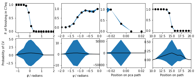
We can use the idea of the isocommittor to identify whether any collective variable is giving a good description of the transition state ensemble's location. The idea in such simulations is to define regions of space that correspond to the various stable states in the free energy landscape. We then launch lots of simulations from configurations that are not within these basins and identify the basin that these calculations visit first. We can then make graphs like those shown below. These graphs show the fraction of times a particular CV value was visited in a trajectory that visited the c7eq basin before it visited the c7ax basin.
The PLUMED input that I used when making the figure above is a filled in version of the following:
phi: TORSION__FILL__=5,7,9,15 psi: TORSIONcould not find this keyword__FILL__=7,9,15,17 pca: PCAVARScould not find this keyword__FILL__=../data/pca-reference.pdbcould not find this keywordTYPE=__FILL__ PRINTcompulsory keyword ( default=OPTIMAL ) The method we are using for alignment to the reference structure__FILL__=phi,psi,pca.eig-1,path.spathcould not find this keywordFILE=colvarthe name of the file on which to output these quantitiesSTRIDE=1 __FILL__compulsory keyword ( default=1 ) the frequency with which the quantities of interest should be outputARG=phicould not find this keywordSTRIDE=1could not find this keywordBASIN_LL1=-3could not find this keywordBASIN_UL1=-1could not find this keywordBASIN_LL2=1could not find this keywordBASIN_UL2=2could not find this keywordFILE=basincould not find this keyword
I deployed the input above within the following python script that launches a large number of gromacs simulations:
Notice how the above script stores the CV values from trajectories that finished in the C7eq basin in the NumPy array called bas_data. We can use the data in this file to construct the (unnormalized) histograms of CV value that finished in C7eq and the total histogram. The script I used to construct these histograms is shown below. This script also shows how we can arrive at the final conditional probability distributions from masterclass21-6-rmsd-committor by dividing by the total number of configurations that moves to C7eq first by the total number of configuration that visited a point.
Notice that the script above does not compute the error bars I included in masterclass21-6-rmsd-committor. Your task in this exercise is to reproduce this figure with the error bars. I generated the error bars in masterclass21-6-rmsd-committor by running 10 sets of 500 simulations. I constructed separate histograms from each of these batches of simulations and calculated the mean and variance from these ten sets of samples.
The exercises in this section aimed to discuss the difference between collective variables and the reaction coordinate. I have argued that collective variables are developed by researchers thinking about coordinates that can distinguish between the important states. Reaction coordinates, meanwhile, are the actual pathways that reactions proceed along. These reaction coordinates are found by probing the data we get from simulations.
I am not convinced that the distinction between reaction coordinates and collective variables is very important. Every coordinate we have tried in the previous sections has allowed us to determine whether we are in the C7eq or the C7ax basin. My view is that when we do science, we impose structure on our results by asking questions. Our question has been to determine the relative free energies of the C7ax and C7eq basins in this exercise. To do this, we have to define what configurations are in the C7ax basin and what configurations are in the C7eq basin. The distinction between these two structures is an arbitrary figment of our imagination. If we use different variables, we might be defining these states differently, and we might get slightly different answers. We should not be surprised by the fact that we get different answers if we ask the question differently. The important thing is to develop an interesting question and to tell a good story about whatever you find out.
Many researchers have used these rare event methods to study nucleation and crystal growth. Studying such problems introduces an additional challenge when designing collective variables as all the atoms are indistinguishable. You thus know before even running the simulation that there are multiple paths that connect the reactant (liquid) state and the product (solid) state. The nucleation, after all, can start with any atom in the simulation box. The first step in developing CVs for studying nucleation processes is thus to identify some order parameter that allows us to distinguish atoms that are in the solid state from atoms that are in the liquid state. The following input, once it is filled in will calculate some suitable order parameters for all the atoms in the system:
UNITSNATURALcoord: COORDINATIONNUMBER( default=off ) use natural units__FILL__=1-5184could not find this keyword__FILL__={CUBIC D_0=1.2 D_MAX=1.5} cub: FCCUBICcould not find this keyword__FILL__=1-5184could not find this keyword__FILL__={CUBIC D_0=1.2 D_MAX=1.5}could not find this keywordALPHA=27 fcub: MTRANSFORM_MOREcompulsory keyword ( default=3.0 ) The alpha parameter of the angular functionDATA=__FILL__compulsory keyword The multicolvar that calculates the set of base quantities that we are interested in__FILL__={SMAP R_0=0.45 D_0=0.0 A=8 B=8} DUMPMULTICOLVARcould not find this keyword__FILL__=coordcould not find this keywordSTRIDE=1000compulsory keyword ( default=1 ) the frequency with which the atoms should be output__FILL_=coord.xyz DUMPMULTICOLVARcould not find this keyword__FILL__=cubcould not find this keywordSTRIDE=1000compulsory keyword ( default=1 ) the frequency with which the atoms should be output__FILL__=cub.xyz DUMPMULTICOLVARcould not find this keyword__FILL__=fcubcould not find this keywordSTRIDE=1000compulsory keyword ( default=1 ) the frequency with which the atoms should be output__FILL__=fcub.xyzcould not find this keyword
You can run a short MD simulation on Lennard-Jonesium to compute those order parameter by using the following input (in) file for simplemd:
inputfile interface.xyz
outputfile output.xyz
temperature 0.6
tstep 0.005
friction 1
forcecutoff 2.5
listcutoff  3.0
nstep 10000
nconfig 100 trajectory.xyz
nstat   100 energies.dat
You can run this from a python notebook and read in the values of the order parameters by using the following script:
A visualization of the order parameters for all the atoms can then be produced using chemiscope, which allows you to see the value of all the individual atom order parameters.
Put all the above together and see if you can produce a chemiscope representation like the one below
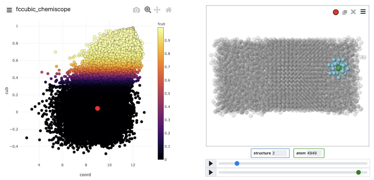
Chemiscope is invaluable for determining whether our order parameter is good at distinguishing the atoms within the solid from those within the liquid. If you visualize the FCCCUBIC or the transformed values of these parameters in the example above, you see that roughly half of the atoms are solid-like, and nearly half of the atoms are liquid-like. Notice also that we can use the dimensionality reduction that were discussed in Exercise 4: Path collective variables and clustering algorithms to develop these atomic order parameters. Generating the data to analyze using these algorithms is easier because we can get multiple sets of coordinates to analyze from each trajectory frame. The atoms are, after all, indistinguishable.
Once we have identified an order parameter we can analyse the distribution of values that it takes by using an input like the one shown below:
UNITSNATURALcoord: COORDINATIONNUMBER( default=off ) use natural units__FILL__=1-5184could not find this keyword__FILL__={CUBIC D_0=1.2 D_MAX=1.5} cub: FCCUBICcould not find this keyword__FILL__=1-5184could not find this keyword__FILL__={CUBIC D_0=1.2 D_MAX=1.5}could not find this keywordALPHA=27 fcub: MTRANSFORM_MOREcompulsory keyword ( default=3.0 ) The alpha parameter of the angular functionDATA=__FILL__compulsory keyword The multicolvar that calculates the set of base quantities that we are interested in__FILL__={SMAP R_0=0.45 D_0=0.0 A=8 B=8} coord_histo: HISTOGRAMcould not find this keyword__FILL__=coordcould not find this keywordSTRIDE=10compulsory keyword ( default=1 ) the frequency with which the data should be collected and added to the quantity being averaged__FILL__=2could not find this keywordGRID_MAX=15compulsory keyword the upper bounds for the grid__FILL__=100could not find this keyword__FILL__=DISCRETE cub_histo: HISTOGRAMcould not find this keyword__FILL__=cubcould not find this keywordSTRIDE=10compulsory keyword ( default=1 ) the frequency with which the data should be collected and added to the quantity being averagedGRID_MIN=-1compulsory keyword the lower bounds for the grid__FILL__=1could not find this keyword__FILL__=100could not find this keyword__FILL__=DISCRETE fcub_histo: HISTOGRAMcould not find this keyword__FILL__=fcubcould not find this keywordSTRIDE=10compulsory keyword ( default=1 ) the frequency with which the data should be collected and added to the quantity being averaged__FILL__=0could not find this keywordGRID_MAX=1compulsory keyword the upper bounds for the grid__FILL__=100could not find this keyword__FILL__=DISCRETE __FILL__could not find this keyword__FILL__=coord_histocould not find this keywordFILE=coord_histo.dat __FILL__could not find this keyword__FILL__=cub_histocould not find this keywordFILE=cub_histo.dat __FILL__could not find this keyword__FILL__=fcub_histocould not find this keywordFILE=fcub_histo.datcould not find this keyword
The resulting distributions of order parameter values should look like this:
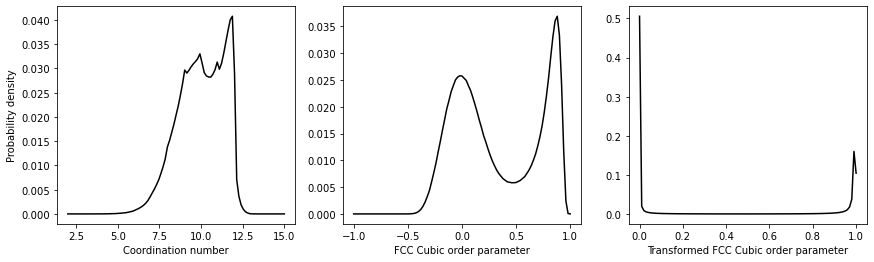
Try to use the information above to reproduce this plot. Notice that the distribution of order parameters for the FCC Cubic order parameters is bimodal. There is a peak corresponding to the value that this quantity takes in the box's liquid part. The second peak then corresponds to the value that the quantity takes in the box's solid part. The same cannot be said for the coordination number by contrast. Notice, last of all, that by transforming the values above we have an order parameter that is one for atoms that are within the solid and zero otherwise.
It is tempting to argue that the number of solid particles is equal to the number of atoms that have an order parameter that is greater than some threshold. A better way to calculate the number of solid particles, however, is to proceed as follows:
Calculate the number of solid \(n_l\) and liquid atoms \(n_l\) by solving the following pair of simultaneous equations \(N=n_s + n_l\) and \(\Phi = n_s \phi_s + n_l \phi_l\), where \(N\) is the total number of atoms. \(\Phi\), meanwhile, is given by:
\[ \Phi = \sum_{i=1}^N \phi_i \]
The sum runs over all the atoms and where \(\phi_i\) is the order parameter for the \(i\)th atom in the system.
This procedure works because \(\Phi\) is an extensive quantity and is thus additive. If we have a system that contains a aolid liquid interface we can express the value of any extensive quantity, \(\Psi\) using:
\[ \Psi = n_s \psi_s + n_l \psi_l + \psi_i \]
where \(\psi_s\) and \(\psi_l\) is the average value per atom value of the quantity \(\psi\) in the solid and liquid phases. \(\psi_i\), meanwhile, is the so-called surface excess term which measures the contribution that the presence of the interface makes to the value of \(\Psi\). When we find \(n_s\) by solving the simultaneous equations above, we assume that this excess term is zero.
To complete this exercise, you should run simulations of the solid, liquid and interface. You should use the ensemble average of the order parameter for your solid and liquid simulations to make a graph like the one below that shows the number of atoms of solid as a function of time for the system that contains the interface. The number of solid atoms has been determined by solving the simultaneous equations using the theory above. Notice that there are input configurations for the solid, liquid and interface systems in the data directory of the GitHub repository. The solid configuration is in solid.xyz. The liquid is in liquid.xyz, and the interface is in interface.xyz. The final result you get will look something like this:
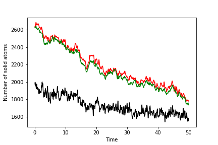
Notice that the green line is the least noisy of these curves. The reason the line is less noisy is connected to the fact that you have the clearest delineation between solid and liquid atoms when you use this order parameter.
NB. We are running at constant volume because we are keeping things simple and using simplemd. If you are studying nucleation using these techniques, you should run at constant pressure.
The exercises in this tutorial have introduced you to the following ideas:
What I would like to do in the follow-up session is to think about how you can use these ideas as you do your research. The first step in using any of these questions is asking a research question that is amenable to answering using one of these methods. In this final exercise, I would like you to think about using these methods in your research. The first step in doing so is asking yourself the question what am I trying to find out? The clearer you make this question, the easier you will find the subsequent research project. With this in mind, here are some examples of terrible research questions:
These research questions are terrible because the final result that you will obtain has not been specified. It is unclear when the project will be finished, or what success in this project looks like. With this in mind, consider the following alternative questions, which each have a clear goal. Each of the goals below maps on to one of the terrible research questions above:
For each of the questions above, it is clear what success will look like – you will have a converged estimate of the free energy difference. We have shown you how such estimates can be extracted in previous masterclasses and what it looks like when such calculations go wrong. Answering these research questions is thus simply a matter of applying what you have learned. Notice, also, how for each of the questions above, it is clear what you can do in the first step:
These simulations may or may not give you the desired free energy difference. You will at least get some trajectory data from them, however. You can then analyze the trajectories using a machine learning algorithm or similar to refine your approach. This refining stage is where the experience of your supervisor should be invaluable.
With all this in mind, think about your research project. Try to develop a research question to work on and an approach that you can use to tackle this question. Your question should not be some grand challenge.
It should be something simple that you know how to do. You do not need to run these simulations. I want you to think about the research question to discuss them at the follow-up session. I want you to think about how you can use these methods in your research as if you are not doing so, attending these masterclasses is pointless as you will never really apply these methods.
 1.8.17