 |
|
|
| |
|
|
The aim of this tutorial is for you to understand how we analyze trajectory data by calculating ensemble averages. One key point we try to make in this tutorial is that you must always calculate averaged quantities from our simulation trajectories. Consequently, in order to understand the analysis that is done when we perform molecular dynamics and Monte Carlo simulations, we will need to understand some things about probability and statistics. In fact, the things that we need to understand about probability and statistics are going to be the main subject of this tutorial. Therefore, in order to make our lives easier, we are not going to work with simulation trajectories in this tutorial. We are going to use model data instead.
Once this tutorial is completed students will:
Let's begin by thinking about what is actually output by a simulation trajectory. You probably know by now that molecular dynamics gives us a trajectory that provides us with information on how the positions and velocities of the all the atoms in the system change with time. Furthermore, you should by now understand that we can use PLUMED to reduce the amount of information contained in each of the trajectory frames to a single number or a low-dimensional vector by calculating a collective variable or a set of collective variables. As we saw in Trieste tutorial: Analyzing trajectories using PLUMED this process of lowering the dimensionality of the data contained in a simulation trajectory was vital as we understand very little by watching the motions of the hundreds of atoms that the system we are simulating contains. If we monitor the appropriate key variables, however, we can determine whether a chemical reaction has taken place, whether the system has undergone a phase transition to a more ordered form or if a protein has folded. Even so if all we do is monitor the values the the collective variables take during the simulation our result can only ever be qualitative and we can only say that we observed this process to take place under these particular conditions on one particular occasion. Obviously, we would like to be able to do more - we would like to be able to make quantitative predictions based on the outcomes of our simulations.
The first step in moving towards making these quantitative predictions involves rethinking what precisely our simulation trajectory has provided us with. We know from rudimentary statistical mechanics that when we perform a molecular dynamics simulation in the NVT ensemble the values of the collective variables that we obtain for each of our trajectory frames, \(X\), are samples from the following probability distribution:
\[ P(s') = \frac{ \int \textrm{d}x \textrm{d}p \delta( s(x) - s') e^{-\frac{H(x,p)}{k_B T}} }{ \int \textrm{d}x\textrm{d}p e^{-\frac{H(x,p)}{k_B T}} } \]
In this expression the integral signs are used to represent \(6N\)-dimensional integrals that run over all the possible positions and momenta that the \(N\) atoms in our system can take. \(H(x,p)\) is the Hamiltonian and \(k_B\) and \(T\) are the Boltzmann constant and the temperature respectively. The quantity calculated by this quotient is the probability that our CV will take a value \(s'\). The quantity in the denominator of the above expression is the canonical partition function while the \(\delta\) function in the integral in the numerator ensures that only those configurations that have a CV value, \(s(x)\), equal to \(s'\) contribute to the integral in the numerator.
The fact that we know what distribution the \(X\)-values obtained from our trajectory frames are taken from is not particularly helpful as it is impossible to calculate the integrals in the expression above analytically. The fact that we know that our trajectory frames represent samples from a distribution is helpful, however, because of a result know as the Central Limit Theorem. This theorem states the following:
\[ \lim_{n \rightarrow \infty} P\left( \frac{\frac{S_n}{n} - \langle Y \rangle}{ \sqrt{\frac{\langle(\delta Y)^2\rangle}{n}} } \le z \right) = \Phi(z) \]
In this expression \(\Phi(z)\) is the cumulative probability distribution function for a standard normal distribution and \(S_n\) is a sum of \(n\) independent samples from a probability distribution - in our case the probability distribution that we introduced in the previous equation. \(\langleY\rangle\) is the ensemble average for the quantity \(Y(x)\), which, in our case, we can calculate as follows:
\[ \langle Y \rangle = \frac{ \int \textrm{d}x \textrm{d}p Y(x) e^{-\frac{H(x,p)}{k_B T}} }{ \int \textrm{d}x\textrm{d}p e^{-\frac{H(x,p)}{k_B T}} } \]
Lastly, the quantity \(\langle(\delta Y)^2\rangle\) is a measure of the extent of the fluctuations we will observe in the \(Y\) values that we samples. This quantity is calculated using:
\[ \langle(\delta Y)^2\rangle = \langle Y^2 \rangle - \langle Y \rangle^2 \]
The statement of the theorem provided above is compact way of stating the formal theorem. This is undoubtedly pleasing to mathematicians but to understand why this idea is so important in the context of molecular simulation it is useful to think about this in a slightly less formal way. The central limit theorem essentially tells us that if we take the set of random variables we extract from a simulation trajectory, which we know represent samples from the complicated distribution in the first equation above, and we add all these random variables together and divide by \(n\) we can think of the final number we obtain as a random variable that is taken from a Gaussian distribution. In other words, the probability density function for the sample mean, \(\frac{S_n}{n}\), that we get from our trajectory frames is given by:
\[ P(S_n) = \frac{1}{\sqrt{\frac{2\pi \langle(\delta Y)^2\rangle}{n}}} \exp\left( - \frac{\frac{S_n}{n} - \langle Y \rangle}{ 2\frac{\langle(\delta Y)^2\rangle}{n} } \right) \]
This function is shown plotted for various values of \(n\) in the movie at https://www.youtube.com/watch?v=-7hlP-2dG_o&feature=youtu.be.
You can see clearly that this distribution becomes more strongly peaked around \(\langle Y\rangle\) (which I set equal to 0 in the movie) as \(n\) increases.
This observation is important as it ensures that the probability that \(\frac{S_n}{n}\) lies close to the true value of the expectation value of our distribution, \(\langle Y\rangle\), increases as we increase the value of \(n\). The central limit theorem therefore allows us to get an estimate for the ensemble average for a particular quantity \(Y\) by taking repeated samples of \(Y\) from our distribution. These samples can be taken by, for example, performing a molecular dynamics simulation. Furthermore, and as we will see in the exercises that follow, we can also get an estimate of how much we might expect the system to fluctuate about this average. Incidentally, if you are confused at this stage you might want to work through these two videos and exercises in order to get a better understanding of the central limit theorem, confidence limits and error bars:
As discussed in the introduction we are going to be using model data in this exercise so we must begin by generating some model data to analyze using PLUMED. The following short python script will generate 10000 (pseudo) random variables between 0 and 1 from a uniform distribution in a format that PLUMED can understand:
Copy the contents of the box above to a plain text file called generate_data.py, save the file and then execute the script within it by running:
> python generate_data.py > my_data
This will generate a file called my_data that contains 10001 uniform random variables. The first few lines of this file should look something like this:
#! FIELDS time rand
0 0.7880696770414992
1 0.6384371499082688
2 0.01373858851099563
3 0.30879241147755776
PLUMED will ignore the first number in the colvar file as it assumes this is the initial configuration you provided for the trajectory. The sample mean will thus be calculated from 10000 random variables. Plot this data now using gnuplot and the command:
gnuplot> p 'my_data' u 1:2 w p
The probability distribution that we generated these random variables is considerably simpler than the probability distribution that we would typically sample from during an MD simulation. Consequently, we can calculate the exact values for the ensemble average and the fluctuations for this distribution. These are:
\[ \begin{aligned} \langle X \rangle &= \int_0^1 x \textrm{d}x = \left[ \frac{x^2}{2} \right]_0^1 = \frac{1}{2} \\ \langle X^2 \rangle &= \int_0^1 x^2 \textrm{d}x = \left[ \frac{x^3}{3} \right]_0^1 = \frac{1}{3} \\ \langle (\delta X)^2 \rangle & = \langle X^2 \rangle - \langle X \rangle^2 = \frac{1}{12} \end{aligned} \]
Lets now try estimating these quantities by calculating \(\frac{S_n}{n}\) from the points we generated and exploiting the central limit theorem. We can do this calculation by writing a PLUMED input file that reads:
data: READFILE=my_datacompulsory keyword the name of the file from which to read these quantitiesVALUES=rand d2: MATHEVALcompulsory keyword the values to read from the fileARG=datathe input for this action is the scalar output from one or more other actions.VAR=athe names to give each of the arguments in the function.FUNC=a*acompulsory keyword the function you wish to evaluatePERIODIC=NO av: AVERAGEcompulsory keyword if the output of your function is periodic then you should specify the periodicity of the function.ARG=datathe input for this action is the scalar output from one or more other actions.STRIDE=1 av2: AVERAGEcompulsory keyword ( default=1 ) the frequency with which the data should be collected and added to the quantity being averagedARG=d2the input for this action is the scalar output from one or more other actions.STRIDE=1 PRINTcompulsory keyword ( default=1 ) the frequency with which the data should be collected and added to the quantity being averagedARG=av,av2the input for this action is the scalar output from one or more other actions.STRIDE=10000compulsory keyword ( default=1 ) the frequency with which the quantities of interest should be outputFILE=colvarthe name of the file on which to output these quantities
If you copy this input to a file called plumed.dat you can then run the calculation by executing:
> plumed driver --noatoms
When the calculation is finished you should have a file called colvar that contains the estimate of the ensemble averages \(\langle X\rangle\) and \(\langle X^2\rangle\). To be clear, the quantities output in this file are:
\[ \langle X \rangle = \frac{1}{N} \sum_{i=1}^N X_i \qquad \textrm{and} \qquad \langle X^2 \rangle \frac{1}{N} \sum_{i=1}^N X_i^2 \]
We can calculate the fluctuations, \((\delta X)^2\), from them using:
\[ (\delta X)^2 = \langle X^2 \rangle - \langle X \rangle^2 \]
We can then compare the values that we got for these estimated values with those that we got for the true values. You should find that the agreement is reasonable but not perfect.
We can use what we have learned about calculating an ensemble average to calculate an estimate for the probability density function or probability mass function for our random variable. The theory behind what we do here is explained in this video http://gtribello.github.io/mathNET/histogram-video.html
To do such a calculation with PLUMED on the random variables we generated from the uniform distribution in the previous section we would use an input like the one below:
data: READFILE=my_datacompulsory keyword the name of the file from which to read these quantitiesVALUES=rand hh: HISTOGRAMcompulsory keyword the values to read from the fileARG=datathe input for this action is the scalar output from one or more other actions.STRIDE=1compulsory keyword ( default=1 ) the frequency with which the data should be collected and added to the quantity being averagedGRID_MIN=0compulsory keyword the lower bounds for the gridGRID_MAX=1.0compulsory keyword the upper bounds for the gridGRID_BIN=20the number of bins for the gridKERNEL=DISCRETE DUMPGRIDcompulsory keyword ( default=gaussian ) the kernel function you are using.GRID=hhcompulsory keyword the action that creates the grid you would like to outputFILE=my_histogram.datcompulsory keyword ( default=density ) the file on which to write the grid.
Once again you can run this calculation by using the command:
> plumed driver --noatoms
Once this calculation is completed you can then plot the output using gnuplot and the command:
gnuplot> p 'my_histogram.dat' u 1:2 w l
In the previous section we compared the estimates we got for the ensemble average with the exact analytical values, which we could determine because we know that the data was sampled from a uniform distribution between 0 and 1. We can do a similar thing with the histogram. Can you determine what the true (analytic) values for the probabilities in the histogram above should be?
Also notice that the probability estimate for the first and last points in our histogram are lower than the probability estimates for the other points.
Can you determine why these two points have a lower probability?
As discussed in previous sections the sample mean of the CV values from our trajectory frames is a random variable and the central limit theorem tells us something about the the distribution from which this random variable is drawn. The fact that we know what distribution the sample mean is drawn from is what allows us to estimate the ensemble average and the fluctuations. The fact that this recipe is only estimating the ensemble average is critical and this realization should always be at the forefront of our minds whenever we analyze our simulation data. The point, once again, is that the sample mean for CV values from the simulation is random. As is explained in this video http://gtribello.github.io/mathNET/central-limit-theorem-video.html, however, we can use the central limit theorem to calculate a range, \(\{\langle X\rangle-\epsilon,\langle X\rangle+\epsilon\}\), that the sample mean for the CV values, \(\frac{S_n}{n}\), will fall into with a probability \(p_c\) using:
\[ \epsilon = \sqrt{ \frac{\langle ( \delta X )^2 \rangle }{n} } \Phi^{-1}\left( \frac{p_c + 1}{2} \right) \]
Here \(\Phi^{-1}\) is the inverse of the cumulative probability distribution function for a normal distribution with mean 0 and variance 1. As you can see this range gets smaller as the number of samples from which you calculate the mean, \(n\), increases. As is shown in the figure below, however, the rate at which this range narrows in size is relatively small.
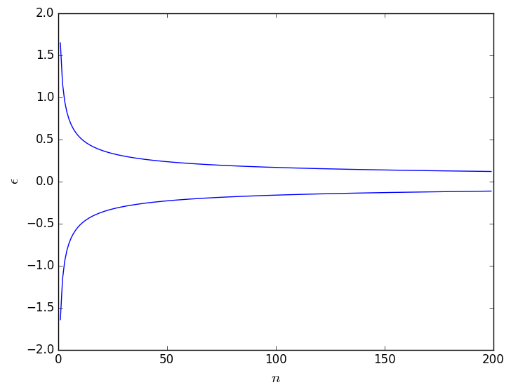
This graph hopefully illustrates to you that an estimate of the ensemble average that is taken over 500 trajectory frames is not guaranteed to lie significantly closer to the true ensemble average than an estimate taken from 100 trajectory frames. For this reason, we might choose to split the data into blocks that all have equal length. Will will then estimate the average for each of these blocks separately. As we will see in the remainder of this exercise this process of block averaging has a number of other advantages. For now though we are just going to use it to test that the results from the various parts of ``the trajectory" are all consistent.
We can perform a block averaging on the data we generated at the start of the first exercise above by using PLUMED and the input file below:
data: READFILE=my_datacompulsory keyword the name of the file from which to read these quantitiesVALUES=rand av: AVERAGEcompulsory keyword the values to read from the fileARG=datathe input for this action is the scalar output from one or more other actions.STRIDE=1compulsory keyword ( default=1 ) the frequency with which the data should be collected and added to the quantity being averagedCLEAR=1000 PRINTcompulsory keyword ( default=0 ) the frequency with which to clear all the accumulated data.ARG=avthe input for this action is the scalar output from one or more other actions.STRIDE=1000compulsory keyword ( default=1 ) the frequency with which the quantities of interest should be outputFILE=colvarthe name of the file on which to output these quantities
Once again this calculation can be executed by running the command:
> plumed driver --noatoms
The key differences between this input and the ones that we have seen previously is the CLEAR keyword on the line AVERAGE. The instruction CLEAR=1000 tells PLUMED that the data that has been accumulated for averaging should be reset to zero (cleared) every 1000 steps. If you look at the subsequent PRINT command in the above input you see the instruction STRIDE=1000. The above input thus accumulates an average over 1000 trajectory frames. This average is then output to the file colvar on step 1000 and the accumulated data is immediately cleared after printing so that a new average over the next 1000 steps can be accumulated. We can plot the averages that were output from the calculation above by using gnuplot and the following command:
gnuplot> p 'colvar' u 1:2 w l
If you try this now you should see that all the average values that were calculated are relatively consistent but that there are differences between them. Try to calculate the size of \(\epsilon\) for a 90 % confidence limit around this random variable using the formula that was provided above. How many of the averages that you extracted using PLUMED lie within this range? Is this behavior inline with your expectations based on your understanding of what a confidence limit is?
We can also perform block averaging when we estimate histograms using PLUMED. The following input will calculate these block averaged histograms for the data we generated at the start of this exercise using PLUMED.
data: READFILE=my_datacompulsory keyword the name of the file from which to read these quantitiesVALUES=rand hh: HISTOGRAMcompulsory keyword the values to read from the fileARG=datathe input for this action is the scalar output from one or more other actions.STRIDE=1compulsory keyword ( default=1 ) the frequency with which the data should be collected and added to the quantity being averagedGRID_MIN=0compulsory keyword the lower bounds for the gridGRID_MAX=1.0compulsory keyword the upper bounds for the gridGRID_BIN=20the number of bins for the gridKERNEL=DISCRETEcompulsory keyword ( default=gaussian ) the kernel function you are using.CLEAR=1000 DUMPGRIDcompulsory keyword ( default=0 ) the frequency with which to clear all the accumulated data.GRID=hhcompulsory keyword the action that creates the grid you would like to outputFILE=my_histogram.datcompulsory keyword ( default=density ) the file on which to write the grid.STRIDE=1000compulsory keyword ( default=0 ) the frequency with which the grid should be output to the file.
Notice that the input here has the same structure as the input for the AVERAGE. Once again we have a CLEAR=1000 keyword that tells PLUMED that the data that has been accumulated for calculating the histogram should be deleted every 1000 steps. In addition, we can set a STRIDE for DUMPGRID and thus output the histogram from each of these blocks of trajectory data separately. The difference between the output from this input and the output from the input above is that in this case we have multiple output files. In particular, the input above should give you 10 output files which will be called:
We can plot all of these histograms using gnuplot and the command:
gnuplot> p 'analysis.0.my_histogram.dat' u 1:2 w l, 'analysis.1.my_histogram.dat' u 1:2 w l, 'analysis.2.my_histogram.dat' u 1:2 w l, 'analysis.3.my_histogram.dat' u 1:2 w l, 'analysis.4.my_histogram.dat' u 1:2 w l, 'analysis.5.my_histogram.dat' u 1:2 w l, 'analysis.6.my_histogram.dat' u 1:2 w l, 'analysis.7.my_histogram.dat' u 1:2 w l, 'analysis.8.my_histogram.dat' u 1:2 w l, 'my_histogram.dat' u 1:2 w l
Performing a comparison between the results from each of these blocks of data is more involved than the analysis we performed when comparing the ensemble averages as we have more data. The essential idea is the same, however, and, if you have time at the end of the session, you might like to see if you can write a script that determines what fraction of the many averages we have calculated here lie within the confidence limits.
As is discussed in many of the tutorials that are provided here one of the primary purposes of PLUMED is to use simulation biases to resolve the rare events problem. When we use these technique we modify the Hamiltonian, \(H(x,p)\), and add to it some bias, \(V(x)\). The modified Hamiltonian thus becomes:
\[ H'(x,p) = H(x,p) + V(x) \]
and as such the values of the collective variables that we obtain from each of our trajectory frames are samples from the following distribution:
\[ P(s') = \frac{ \int \textrm{d}x \textrm{d}p \delta( s(x) - s') e^{-\frac{H(x,p)}{k_B T}}e^{-\frac{V(x)}{k_B T}} }{ \int \textrm{d}x\textrm{d}p e^{-\frac{H(x,p)}{k_B T}}e^{-\frac{V(x)}{k_B T}} } \]
Using a bias in this way is enormously helpful as we can ensure that we sample from a particular part of configuration space. We appear to have sacrificed, however, the ability to extract estimates of ensemble averages for the unbiased distribution using the central limit theorem. If we calculate the mean from a set of trajectory frames that are sampled from the distribution above we will get an estimate for the ensemble average in this biased distribution. As we will see in this exercise, however, this is not really a problem as we can use reweighting techniques to extract ensemble averages for the unbiased distribution.
Lets begin by generating some new trajectory data. The following python script generates a set of random variables from a (truncated) normal distribution with \(\sigma=0.5\) and \(\mu=0.6\). In other words, points are generated from the following probability distribution but if they don't fall in a range between 0 and 1 they are discarded:
\[ P(x) = \frac{1}{\sqrt{2\pi}\sigma} \exp\left(-\frac{(x-\mu)^2}{2\sigma^2}\right) \]
Copy the script above to a file called gen-normal.py and then execute the python script within it using the command:
> python gen-normal.py > normal_data
This should produce a file called normal_data. The first few lines of this file will look something like the following:
#! FIELDS time rand
0 0.7216627600374712
1 0.7460765782434674
2 0.7753011891527442
3 0.5643419178297695
Use what you have learned from the exercises above to estimate the ensemble average from these generated data points using PLUMED. If you want you can use block averaging but it does not matter if you do it by just considering all the data in the input file. What would you expect the ensemble average to be and how does the estimate you get from PLUMED compare with the true value?
You should have found that the ensemble average that you get when you perform the experiment described in the previous paragraph is different from the ensemble average that you get when you considered the uniform distribution. This makes sense as the distribution we sampled from here is approximately:
\[ P(x) = \frac{1}{0.03*\sqrt{2\pi}} \exp\left( - \frac{ x - 0.6}{ 2(0.03)^2} \right) \]
This is different from the distribution we sampled from in the previous exercises. A question we might therefore ask is: can we extract the ensemble average for the uniform distribution that we sampled in previous exercises by sampling from this different distribution? In the context of the experiment we are performing here with the random variables this question perhaps feels somewhat absurd and pointless. In the context of molecular simulation, however, answering this question is essential as our ability to extract the true, unbiased distribution from a simulation run with a bias relies on being able to perform this sort of reweighting.
The true value of the ensemble average, which we estimated when we analyzed the data generated from the Gaussian using the python script above is given by:
\[ \langle X \rangle = \frac{ \int_0^1 x e^{-V(x)} \textrm{d}x }{\int_0^1 e^{-V(x)} \textrm{d}x } \qquad \textrm{where} \qquad V(x) = \frac{ (x - x)^2}{2\sigma^2} \]
By contrast the ensemble average in the exercises involving the uniform distribution is given by:
\[ \langle Y \rangle = \frac{ \int_0^1 y \textrm{d}y }{ \int_0^1 \textrm{d}y } = \frac{ \int_0^1 y e^{-V(y)}e^{+V(y)} \textrm{d}y }{\int_0^1 e^{-V(y)}e^{+V(y)} \textrm{d}y } \]
We can use the final expression here to reweight the data that we sampled from the Gaussian. By doing so can thus extract ensemble averages for the uniform distribution. The trick here is calculate the following weighted mean rather than the unweighted mean that we calculated previously:
\[ \langle Y \rangle \approx \frac{\sum_i Y_i e^{+V(Y_i)}}{ \sum_i e^{+V(Y_i)} } \]
where here the sums run over all the random variables, the \(Y_i\)s, that we sampled from the Gaussian distribution. If you used the script above the \(V(Y_i)\) values were output for you so you can calculate this estimate of the ensemble average for the unbiased distribution in this case using the following PLUMED input.
UNITSNATURAL# This ensures that Boltzmann's constant is one data: READ( default=off ) use natural unitsFILE=normal_datacompulsory keyword the name of the file from which to read these quantitiesVALUES=randcompulsory keyword the values to read from the fileIGNORE_FORCESmm: RESTRAINT( default=off ) use this flag if the forces added by any bias can be safely ignored.ARG=datathe input for this action is the scalar output from one or more other actions.AT=0.6compulsory keyword the position of the restraintKAPPA=33.333 rw: REWEIGHT_BIAScompulsory keyword ( default=0.0 ) specifies that the restraint is harmonic and what the values of the force constants on each of the variables areTEMP=1 av: AVERAGEthe system temperature.ARG=datathe input for this action is the scalar output from one or more other actions.STRIDE=1compulsory keyword ( default=1 ) the frequency with which the data should be collected and added to the quantity being averagedLOGWEIGHTS=rw PRINTlist of actions that calculates log weights that should be used to weight configurations when calculating averagesARG=avthe input for this action is the scalar output from one or more other actions.STRIDE=10000compulsory keyword ( default=1 ) the frequency with which the quantities of interest should be outputFILE=colvarthe name of the file on which to output these quantities
Try to run this calculation now using:
> plumed driver --noatoms
and see how close you get to the ensemble average for the uniform distribution. Once you have done this try the following input, which allows you to compute the reweighted histogram.
UNITSNATURAL# This ensures that Boltzmann's constant is one data: READ( default=off ) use natural unitsFILE=normal_datacompulsory keyword the name of the file from which to read these quantitiesVALUES=randcompulsory keyword the values to read from the fileIGNORE_FORCESmm: RESTRAINT( default=off ) use this flag if the forces added by any bias can be safely ignored.ARG=datathe input for this action is the scalar output from one or more other actions.AT=0.6compulsory keyword the position of the restraintKAPPA=33.333 rw: REWEIGHT_BIAScompulsory keyword ( default=0.0 ) specifies that the restraint is harmonic and what the values of the force constants on each of the variables areTEMP=1 hh: HISTOGRAMthe system temperature.ARG=datathe input for this action is the scalar output from one or more other actions.STRIDE=1compulsory keyword ( default=1 ) the frequency with which the data should be collected and added to the quantity being averagedGRID_MIN=0compulsory keyword the lower bounds for the gridGRID_MAX=1.0compulsory keyword the upper bounds for the gridGRID_BIN=20the number of bins for the gridKERNEL=DISCRETEcompulsory keyword ( default=gaussian ) the kernel function you are using.LOGWEIGHTS=rw DUMPGRIDlist of actions that calculates log weights that should be used to weight configurations when calculating averagesGRID=hhcompulsory keyword the action that creates the grid you would like to outputFILE=my_histogram.datcompulsory keyword ( default=density ) the file on which to write the grid.
Plot the histogram that you obtain from this calculation using the command:
gnuplot> p 'my_histogram.dat' w l
Now suppose that the data we generated for this exercise had come from an MD simulation. What would the unbiased Hamiltonian in this MD simulation have looked like and what functional form would our simulation bias have taken?
As a good scientist you have probably noticed that we have failed to provide error bars around our estimates for the ensemble average in previous sections. Furthermore, you may have found that rather odd given that I showed you how to estimate the variance in the data in the very first exercise. This ignoring of the error bars has been deliberate, however, as there is a further problem with the data that comes from molecular dynamics trajectories that we have to learn to deal with and that will affect our ability to estimate the error bars. This problem is connected to the fact that the central limit theorem only holds when we take a sum of uncorrelated and identical random variables. Random variables that are generated from simulation trajectories will contain correlations simply because the system will most likely not diffuse from one edge of CV space to the other during a single timestep. In other words, the random CV value that we calculate from the \((i+1)\)th frame of the trajectory will be similar to the value obtained from the \(i\)th trajectory frame. This problem can be resolved, however, and to show how we will thus use the following python script to generate some correlated model data:
Copy the python script above to a filled called correlated-data.py and then execute the script using the command:
> python correlated-data.py > correlated_data
This should output a file called correlated_data. The first few lines of this file should look something like the following:
#! FIELDS time rand
0 0.17818391042061332
1 0.33368077871483476
2 0.0834749323925259
The autocorrelation function, \(R(\tau)\) provides a simple method for determining whether or not there are correlations between the random variables, \(X\), in our time series. This function is defined as follows:
\[ R(\tau) = \frac{ \langle (X_t - \langle X \rangle )(X_{t+\tau} - \langle X \rangle ) \rangle }{ \langle (\delta X)^2 \rangle } \]
At present it is not possible to calculate this function using PLUMED. If we were to do so for the samples taken from the uniform distribution and the correlated samples that were taken from the distribution the python script above we would find that the auto correlation functions for these random variables look something like the figures shown below:
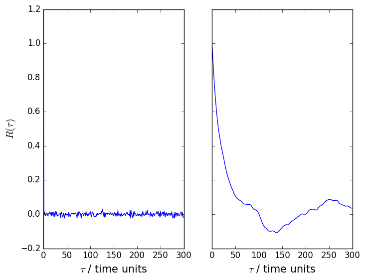
To understand what these functions are telling us lets deal with the samples from the uniform distribution first. The autocorrelation function in this case has a value of 1 when \(\tau\) is equal to 0 and a value of 0 in all other cases. This function thus tells us that each random variable is perfectly correlated with itself but that there are no correlations between the distributions we sampled adjacent variables from. In other words, each of the random variables we generate are independent. If we now look at the autocorrelation function for the distribution that is sampled by the python script above we see that the autocorrelation function slowly decays to zero. There are, therefore, correlations between the random variables that we generate that we must account for when we perform our analysis.
We account for the correlations in the data when we do our analysis by performing a block analysis. To understand what precisely this involves we are going to perform the analysis with PLUMED and explain the results that we get at each stage of the process. We will begin by analyzing the data we generated by sampling from the uniform distribution using the following PLUMED input:
data: READFILE=correlated_datacompulsory keyword the name of the file from which to read these quantitiesVALUES=rand av5: AVERAGEcompulsory keyword the values to read from the fileARG=datathe input for this action is the scalar output from one or more other actions.STRIDE=1compulsory keyword ( default=1 ) the frequency with which the data should be collected and added to the quantity being averagedCLEAR=5 PRINTcompulsory keyword ( default=0 ) the frequency with which to clear all the accumulated data.ARG=av5the input for this action is the scalar output from one or more other actions.FILE=colvar5the name of the file on which to output these quantitiesSTRIDE=5 av10: AVERAGEcompulsory keyword ( default=1 ) the frequency with which the quantities of interest should be outputARG=datathe input for this action is the scalar output from one or more other actions.STRIDE=1compulsory keyword ( default=1 ) the frequency with which the data should be collected and added to the quantity being averagedCLEAR=10 PRINTcompulsory keyword ( default=0 ) the frequency with which to clear all the accumulated data.ARG=av10the input for this action is the scalar output from one or more other actions.FILE=colvar10the name of the file on which to output these quantitiesSTRIDE=10 av15: AVERAGEcompulsory keyword ( default=1 ) the frequency with which the quantities of interest should be outputARG=datathe input for this action is the scalar output from one or more other actions.STRIDE=1compulsory keyword ( default=1 ) the frequency with which the data should be collected and added to the quantity being averagedCLEAR=15 PRINTcompulsory keyword ( default=0 ) the frequency with which to clear all the accumulated data.ARG=av15the input for this action is the scalar output from one or more other actions.FILE=colvar15the name of the file on which to output these quantitiesSTRIDE=15 av20: AVERAGEcompulsory keyword ( default=1 ) the frequency with which the quantities of interest should be outputARG=datathe input for this action is the scalar output from one or more other actions.STRIDE=1compulsory keyword ( default=1 ) the frequency with which the data should be collected and added to the quantity being averagedCLEAR=20 PRINTcompulsory keyword ( default=0 ) the frequency with which to clear all the accumulated data.ARG=av20the input for this action is the scalar output from one or more other actions.FILE=colvar20the name of the file on which to output these quantitiesSTRIDE=20 av25: AVERAGEcompulsory keyword ( default=1 ) the frequency with which the quantities of interest should be outputARG=datathe input for this action is the scalar output from one or more other actions.STRIDE=1compulsory keyword ( default=1 ) the frequency with which the data should be collected and added to the quantity being averagedCLEAR=25 PRINTcompulsory keyword ( default=0 ) the frequency with which to clear all the accumulated data.ARG=av25the input for this action is the scalar output from one or more other actions.FILE=colvar25the name of the file on which to output these quantitiesSTRIDE=25 av30: AVERAGEcompulsory keyword ( default=1 ) the frequency with which the quantities of interest should be outputARG=datathe input for this action is the scalar output from one or more other actions.STRIDE=1compulsory keyword ( default=1 ) the frequency with which the data should be collected and added to the quantity being averagedCLEAR=30 PRINTcompulsory keyword ( default=0 ) the frequency with which to clear all the accumulated data.ARG=av30the input for this action is the scalar output from one or more other actions.FILE=colvar30the name of the file on which to output these quantitiesSTRIDE=30 av35: AVERAGEcompulsory keyword ( default=1 ) the frequency with which the quantities of interest should be outputARG=datathe input for this action is the scalar output from one or more other actions.STRIDE=1compulsory keyword ( default=1 ) the frequency with which the data should be collected and added to the quantity being averagedCLEAR=35 PRINTcompulsory keyword ( default=0 ) the frequency with which to clear all the accumulated data.ARG=av35the input for this action is the scalar output from one or more other actions.FILE=colvar35the name of the file on which to output these quantitiesSTRIDE=35 av40: AVERAGEcompulsory keyword ( default=1 ) the frequency with which the quantities of interest should be outputARG=datathe input for this action is the scalar output from one or more other actions.STRIDE=1compulsory keyword ( default=1 ) the frequency with which the data should be collected and added to the quantity being averagedCLEAR=40 PRINTcompulsory keyword ( default=0 ) the frequency with which to clear all the accumulated data.ARG=av40the input for this action is the scalar output from one or more other actions.FILE=colvar40the name of the file on which to output these quantitiesSTRIDE=40 av45: AVERAGEcompulsory keyword ( default=1 ) the frequency with which the quantities of interest should be outputARG=datathe input for this action is the scalar output from one or more other actions.STRIDE=1compulsory keyword ( default=1 ) the frequency with which the data should be collected and added to the quantity being averagedCLEAR=45 PRINTcompulsory keyword ( default=0 ) the frequency with which to clear all the accumulated data.ARG=av45the input for this action is the scalar output from one or more other actions.FILE=colvar45the name of the file on which to output these quantitiesSTRIDE=45 av50: AVERAGEcompulsory keyword ( default=1 ) the frequency with which the quantities of interest should be outputARG=datathe input for this action is the scalar output from one or more other actions.STRIDE=1compulsory keyword ( default=1 ) the frequency with which the data should be collected and added to the quantity being averagedCLEAR=50 PRINTcompulsory keyword ( default=0 ) the frequency with which to clear all the accumulated data.ARG=av50the input for this action is the scalar output from one or more other actions.FILE=colvar50the name of the file on which to output these quantitiesSTRIDE=50 av55: AVERAGEcompulsory keyword ( default=1 ) the frequency with which the quantities of interest should be outputARG=datathe input for this action is the scalar output from one or more other actions.STRIDE=1compulsory keyword ( default=1 ) the frequency with which the data should be collected and added to the quantity being averagedCLEAR=55 PRINTcompulsory keyword ( default=0 ) the frequency with which to clear all the accumulated data.ARG=av55the input for this action is the scalar output from one or more other actions.FILE=colvar55the name of the file on which to output these quantitiesSTRIDE=55 av60: AVERAGEcompulsory keyword ( default=1 ) the frequency with which the quantities of interest should be outputARG=datathe input for this action is the scalar output from one or more other actions.STRIDE=1compulsory keyword ( default=1 ) the frequency with which the data should be collected and added to the quantity being averagedCLEAR=60 PRINTcompulsory keyword ( default=0 ) the frequency with which to clear all the accumulated data.ARG=av60the input for this action is the scalar output from one or more other actions.FILE=colvar60the name of the file on which to output these quantitiesSTRIDE=60 av65: AVERAGEcompulsory keyword ( default=1 ) the frequency with which the quantities of interest should be outputARG=datathe input for this action is the scalar output from one or more other actions.STRIDE=1compulsory keyword ( default=1 ) the frequency with which the data should be collected and added to the quantity being averagedCLEAR=65 PRINTcompulsory keyword ( default=0 ) the frequency with which to clear all the accumulated data.ARG=av65the input for this action is the scalar output from one or more other actions.FILE=colvar65the name of the file on which to output these quantitiesSTRIDE=65 av70: AVERAGEcompulsory keyword ( default=1 ) the frequency with which the quantities of interest should be outputARG=datathe input for this action is the scalar output from one or more other actions.STRIDE=1compulsory keyword ( default=1 ) the frequency with which the data should be collected and added to the quantity being averagedCLEAR=70 PRINTcompulsory keyword ( default=0 ) the frequency with which to clear all the accumulated data.ARG=av70the input for this action is the scalar output from one or more other actions.FILE=colvar70the name of the file on which to output these quantitiesSTRIDE=70compulsory keyword ( default=1 ) the frequency with which the quantities of interest should be output
Copy the input above to a file called plumed.dat and run the calculation using the command:
> plumed driver --noatoms
This calculation should output 14 colvar files, which should then be further analyzed using the following python script:
Copy this script to a file called block-average-script.py and then execute the contents using the command:
> python block-average-script.py > my_averages.dat
This will output a single file called my_averages.dat that can be plotted using gnuplot and the command:
gnuplot> p 'my_averages.dat' u 1:2:3 w e, 'my_averages.dat' w l
The final result should be a graph like that shown in the left panel of the figure below. The figure on the right shows what you should obtain when you repeat the same analysis on the correlated data that we generated using the python script in this section.
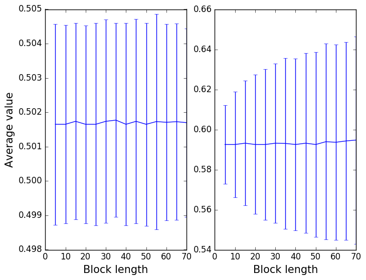
The output that you obtain from these two calculations is explained in the video at: http://gtribello.github.io/mathNET/block_averaging_video.html Before watching this explanation though take some time to note down the differences between the two graphs above. Try to look through the scripts above and to understand what is being done in the PLUMED inputs and the python scripts above so as to work out what the data in these two figures are telling you.
In this final exercise we are going to try to combine everything we have seen in the previous sections. We are going to sample from the distribution that was introduced in Problem II: Dealing with rare events and simulation biases. This time though we are not going to generate random variables from the Gaussian directly. We are instead going to use Monte Carlo sampling. This sampling method is going to give us correlated data so we will need to use ideas from Problem III: Dealing with correlated variables in order to get a proper estimate of the error bars. Furthermore, we are not going to try to extract ensemble averages that tell us about the distribution we sampled from. Instead we are going to reweight using the ideas from Problem II: Dealing with rare events and simulation biases and extract the unbiased distribution.
The first step in doing all this is, as always, to generate some data. The python script below will generate this data:
Copy this script to a filled called do-monte-carlo.py and execute the contents of the script using the command:
> python do-monte-carlo.py > monte_carlo_data
This will run a short Monte Carlo simulation that generates (time-correlated) random data from a (roughly) Gaussian distribution by attempting random translational moves of up to 0.1 units. The command above will generate a file called monte_carlo_data the first few lines of which should look something like the following:
#! FIELDS time rand
0 0.17818391042061332
1 0.33368077871483476
2 0.0834749323925259
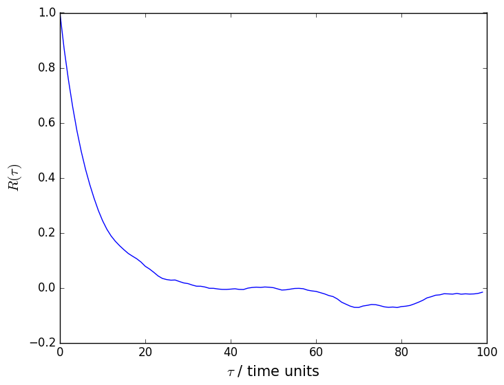
An autocorrelation function that was calculated using data generated using this script is shown below. You can clearly see from this figure that there are correlations between the adjacent data points in the time series and that we have to do block averaging as a result.
We can use the following PLUMED input to calculate block averages for the unbiased histogram from the data we generated:
UNITSNATURAL# This ensures that Boltzmann's constant is one data: READ( default=off ) use natural unitsFILE=monte_carlo_datacompulsory keyword the name of the file from which to read these quantitiesVALUES=randcompulsory keyword the values to read from the fileIGNORE_FORCESmm: RESTRAINT( default=off ) use this flag if the forces added by any bias can be safely ignored.ARG=datathe input for this action is the scalar output from one or more other actions.AT=0.6compulsory keyword the position of the restraintKAPPA=33.333 rw: REWEIGHT_BIAScompulsory keyword ( default=0.0 ) specifies that the restraint is harmonic and what the values of the force constants on each of the variables areTEMP=1 hh: HISTOGRAMthe system temperature.ARG=datathe input for this action is the scalar output from one or more other actions.STRIDE=1compulsory keyword ( default=1 ) the frequency with which the data should be collected and added to the quantity being averagedGRID_MIN=0compulsory keyword the lower bounds for the gridGRID_MAX=1.0compulsory keyword the upper bounds for the gridGRID_BIN=20the number of bins for the gridKERNEL=DISCRETEcompulsory keyword ( default=gaussian ) the kernel function you are using.LOGWEIGHTS=rwlist of actions that calculates log weights that should be used to weight configurations when calculating averagesCLEAR=500 DUMPGRIDcompulsory keyword ( default=0 ) the frequency with which to clear all the accumulated data.GRID=hhcompulsory keyword the action that creates the grid you would like to outputFILE=my_histogram.datcompulsory keyword ( default=density ) the file on which to write the grid.STRIDE=500compulsory keyword ( default=0 ) the frequency with which the grid should be output to the file.
Notice that this input instructs PLUMED to calculate block averages for the histogram from each set of 500 consecutive frames in the trajectory.
I have worked out that this is an appropriate length of time to average over by performing the analysis described in Problem III: Dealing with correlated variables.
We will come back to how precisely I did this momentarily, however. For the time being though you can execute this input using:
> plumed driver --noatoms
Executing this command will generate a number of files containing histograms. The following python script will merge all this data and calculate the final histogram together with the appropriate error bars.
Copy this script to a file called merge-histograms.py and then run its contents by executing the command:
> python merge-histograms.py > final-histogram.dat
This will output the final average histogram together with some error bars. You can plot this function using gnuplot by executing the command:
gnuplot> p 'final-histogram.dat' u 1:2:3 w e, '' u 1:2 w l
Where are the error bars in our estimate of the histogram the largest? Why are the errors large in these regions?
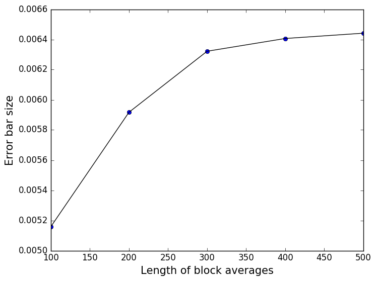
Notice that the file output by the script above also contains information on the average error per grid point in the header. The quantity that is calculated here is:
\[ \textrm{average error} = \frac{1}{N} \sum_{i=1}^N \sigma_i \]
In this expression \(N\) is the total number of grid points at which the function was evaluated and \(\sigma_i\) is the error bar for the estimate of the function that was calculated for the \(i\)th grid point. The average error is a useful quantity as we can plot it and thus check that our blocks are large enough to correct for the correlation between our data points. In other words, we can use this quantity in the same way that we used the error around the average in Problem III: Dealing with correlated variables. A plot of the average error versus the size of the blocks that were used in for the block averaging is shown below. This figure demonstrates that a block average length of 500 is certainly long enough to correct for the problems due to the correlations in the values produced at different times:
If you have sufficient time try to see if you can reproduce this plot using the data you generated
The exercises in the previous sections have shown you how we can calculate ensemble averages from trajectory data. You should have seen that performing block averaging is vital as this technique allows us to deal with the artifacts that we get because of the correlations in the data that we obtain from simulation trajectories.
What we have seen is that when this technique is used correctly we get reasonable error bars. If block averaging is not performed, however, we can underestimate the errors in our data and thus express a false confidence in the reliability of our simulation results.
The next step for you will be to use this technique when analyzing the data from your own simulations.
 1.8.17