 |
|
|
| |
|
|
The aim of this tutorial is to introduce the use of VES for obtaining kinetic information of activated processes. We will learn how to set up a biased simulation using a fixed flooding potential acting on a relevant slow degree of freedom. We can then scale the accelerated MD time in a post-processing procedure.
Once this tutorial is completed students will:
The tarball for this project contains the following files:
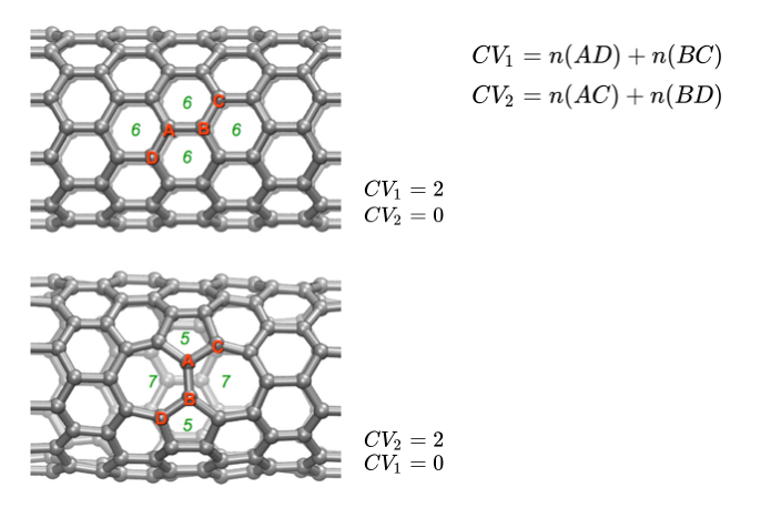
As an example of an activated process in materials science, we will work with the Stone-Wales transformation in a carbon nanotube. The tarball for this project contains the inputs necessary to run a simulation in LAMMPS for a 480 atom carbon nanotube. We use the AIREBO (Adaptive Intermolecular Reactive Empirical Bond Order) force field parameters which can approximately describe C-C bond breakage and formation at reasonable computational cost. For CVs we can use the coordination number in PLUMED to measure the number of covalent bonds among different groups of atoms. The transformation involves breaking two C-C bonds and forming two alternative C-C bonds.A definition of these CVs as well as the relevant C-C bonds are depicted in Figure stone-wales. We prepare a PLUMED input file as follows.
# set distance units to angstrom, time to ps, and energy to eV UNITSLENGTH=Athe units of lengths.TIME=psthe units of time.ENERGY=eV # define two variables CV1: COORDINATIONthe units of energy.GROUPA=229,219First list of atoms.GROUPB=238,207Second list of atoms (if empty, N*(N-1)/2 pairs in GROUPA are counted).R_0=1.8could not find this keywordNN=8compulsory keyword ( default=6 ) The n parameter of the switching functionMM=16compulsory keyword ( default=0 ) The m parameter of the switching function; 0 implies 2*NNPAIRCV2: COORDINATION( default=off ) Pair only 1st element of the 1st group with 1st element in the second, etcGROUPA=229,219First list of atoms.GROUPB=207,238Second list of atoms (if empty, N*(N-1)/2 pairs in GROUPA are counted).R_0=1.8could not find this keywordNN=8compulsory keyword ( default=6 ) The n parameter of the switching functionMM=16compulsory keyword ( default=0 ) The m parameter of the switching function; 0 implies 2*NNPAIR# the difference between variables d1: COMBINE( default=off ) Pair only 1st element of the 1st group with 1st element in the second, etcARG=CV1,CV2the input for this action is the scalar output from one or more other actions.COEFFICIENTS=1,-1compulsory keyword ( default=1.0 ) the coefficients of the arguments in your functionPOWERS=1,1compulsory keyword ( default=1.0 ) the powers to which you are raising each of the arguments in your functionPERIODIC=NOcompulsory keyword if the output of your function is periodic then you should specify the periodicity of the function.
In the above, the first line sets the energy units. The second and third line define the two CVs for the C-C covalent bonds. (We have chosen atoms 238,207,229 and 219; however this choice is arbitrary and other atoms could equally well have been chosen.) Lastly, we define a simple approximate reaction coordinate given by the difference between CV1 and CV2 that we can use to monitor the transition.
Next we will use VES to drive the transformation at 1700 K. We bias the formation of bonds DB and AC shown in Figure stone-wales using CV2 which changes from 0 to 2 during the transformation. (Although a more rigorous treatment would bias both CVs, for this tutorial we will simplify things and work in only one dimension). We choose a Chebyshev polynomial basis set up to order 36
__FILL__ # The basis set to use bf1: BF_CHEBYSHEVORDER=36compulsory keyword The order of the basis function expansion.MINIMUM=0.0compulsory keyword The minimum of the interval on which the basis functions are defined.MAXIMUM=2.0compulsory keyword The maximum of the interval on which the basis functions are defined.
and we tell PLUMED to use VES acting on CV2 with a free energy cutoff
__FILL__ td_uniform: TD_UNIFORM variational: VES_LINEAR_EXPANSION ...ARG=CV2the input for this action is the scalar output from one or more other actions.BASIS_FUNCTIONS=bf1compulsory keyword the label of the one dimensional basis functions that should be used.TEMP=1700the system temperature - this is needed if the MD code does not pass the temperature to PLUMED.BIAS_CUTOFF=15.0cutoff the bias such that it only fills the free energy surface up to certain level F_cutoff, here you should give the value of the F_cutoff.BIAS_CUTOFF_FERMI_LAMBDA=10.0the lambda value used in the Fermi switching function for the bias cutoff (BIAS_CUTOFF), the default value is 10.0.TARGET_DISTRIBUTION=td_uniform ...the label of the target distribution to be used.
Here we are biasing CV2 with the basis set defined above. The final two lines impose the cutoff at 15 eV. The cutoff is of the form
\[ \frac{1}{1+e^{\lambda [F(s)-F_c]}} \]
where \(\lambda\) (inverse energy units) controls how sharply the function goes to zero. Above we have set \(\lambda=10.0\) to ensure the cutoff goes sharply enough to zero.
The following input updates the VES bias every 200 steps, writing out the bias every 10 iterations. To enforce the energy cutoff we also need to update the target distribution which we do every 40 iterations with the TARGETDIST_STRIDE flag.
__FILL__ var-S: OPT_AVERAGED_SGD ...BIAS=variationalcompulsory keyword the label of the VES bias to be optimizedSTRIDE=200compulsory keyword the frequency of updating the coefficients given in the number of MD steps.STEPSIZE=0.1compulsory keyword the step size used for the optimizationCOEFFS_FILE=coeffs.datcompulsory keyword ( default=coeffs.data ) the name of output file for the coefficientsBIAS_OUTPUT=10how often the bias(es) should be written out to file.TARGETDIST_STRIDE=40stride for updating a target distribution that is iteratively updated during the optimization.TARGETDIST_OUTPUT=40how often the dynamic target distribution(s) should be written out to file.COEFFS_OUTPUT=1 ...compulsory keyword ( default=100 ) how often the coefficients should be written to file.
Finally, we will stop the simulation when the transition occurs using the COMMITTOR in PLUMED
__FILL__ COMMITTORARG=d1the input for this action is the scalar output from one or more other actions.BASIN_LL1=-2.0compulsory keyword List of lower limits for basin # You can use multiple instances of this keyword i.e.BASIN_UL1=-1.0compulsory keyword List of upper limits for basin # You can use multiple instances of this keyword i.e.STRIDE=600compulsory keyword ( default=1 ) the frequency with which the CVs are analyzed
Run the simulation using LAMMPS
lmp_mpi < input
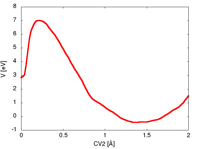
and plot the last few bias output files (bias.variational.iter-n.data) using gnuplot. What is the difference between the maximum and minimum values of the bias obtained during the simulation? Is the cutoff value sufficient to cross the barrier? Is the cutoff value too large?
Figure Figure1A shows an example bias potential after 90 iterations. Note that a cutoff of 15 eV is too large as the system transitions before the bias reaches the prescribed cutoff. From Figure Figure1A we see a barrier height of approximately 7.3 eV.
The output also produces an movie.xyz file which can be viewed in vmd. For better visualization, first change atom id from 1 to C by typing
sed "s/^1 /C /" movie.xyz > newmovie.xyz
Then load the newmovie.xyz into vmd and choose Graphics --> Representations and set Drawing Method to DynamicBonds. Create a second representation by clicking Create Rep and set the Drawing Method to VDW. Change the sphere scale to 0.3 and play the movie. You should observe the Stone-Wales transformation right before the end of the trajectory.
In this exercise we will run a VES simulation to fill the FES only up to a certain cutoff. This will be the first step in order to obtain kinetic information from biased simulations. In the previous section, we observed that a cutoff of 15 eV is too strong for our purpose. Change the cutoff energy from 15.0 to 6.0 eV by setting
BIAS_CUTOFF=6.0
and rerun the simulation from Exercise 1A. [Note: In practice one can use multiple walkers during the optimization by adding the flag MULTIPLE_WALKERS]
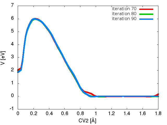
Plot some of the bias files (bias.variational.iter-n.data) that are printed during the simulation using gnuplot. At the end of the simulation, you should be able to reproduce something like Figure Figure1B. Is the bias converging? If so, how many iterations does it require to converge?
Figure Figure1B shows the bias potential after 70,80, and 90 iteration steps. Note that the bias has reached the cutoff and goes to zero at around 1 Angstrom.
In this exercise we will use the bias obtained above as a static umbrella potential. We will set up and run a new trajectory to measure the first passage time of escape from the well.
We can extract the coefficients that we need from the final iteration in Exercise-1B above.
tail -n 47 coeffs.dat > fixed-coeffs.dat
Now create a new directory from which you will run a new simulation and copy the necessary input files (including the fixed-coeffs.dat) into this directory. Modify the PLUMED file so that the optimized coefficients are read by the VES_LINEAR_EXPANSION
__FILL__ td_uniform: TD_UNIFORM variational: VES_LINEAR_EXPANSION ...ARG=CV2the input for this action is the scalar output from one or more other actions.BASIS_FUNCTIONS=bf1compulsory keyword the label of the one dimensional basis functions that should be used.TEMP=1700the system temperature - this is needed if the MD code does not pass the temperature to PLUMED.BIAS_CUTOFF=6.0cutoff the bias such that it only fills the free energy surface up to certain level F_cutoff, here you should give the value of the F_cutoff.BIAS_CUTOFF_FERMI_LAMBDA=10.0the lambda value used in the Fermi switching function for the bias cutoff (BIAS_CUTOFF), the default value is 10.0.TARGET_DISTRIBUTION=td_uniformthe label of the target distribution to be used.COEFFS=fixed-coeffs.dat ...read in the coefficients from files.
The final line specifies the coefficients to be read from a file.
Make sure to remove the lines for the stochastic optimization (OPT_AVERAGED_SGD) as we no longer wish to update the bias.
We will also perform metadynamics with an infrequent deposition stride to ensure that the trajectory does not get stuck in any regions where the bias potential is not fully converged The following implements metadynamics on both CV1 and CV2 with a deposition stride of 4000 steps and a hill height of 0.15 eV.
__FILL__ metad: METAD ...ARG=CV1,CV2the input for this action is the scalar output from one or more other actions.SIGMA=0.2,0.2compulsory keyword the widths of the Gaussian hillsHEIGHT=0.15the heights of the Gaussian hills.PACE=4000 ...compulsory keyword the frequency for hill addition
Again we will use the COMMITTOR to stop the trajectory after the transition.
__FILL__ COMMITTORARG=d1the input for this action is the scalar output from one or more other actions.BASIN_LL1=-2.0compulsory keyword List of lower limits for basin # You can use multiple instances of this keyword i.e.BASIN_UL1=-1.0compulsory keyword List of upper limits for basin # You can use multiple instances of this keyword i.e.
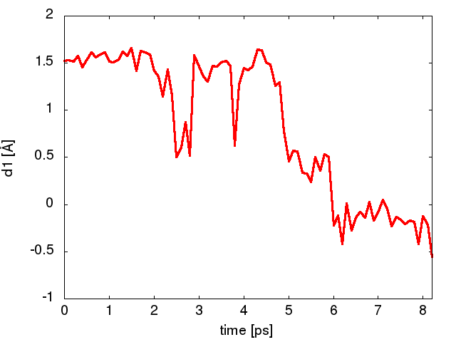
Now run a trajectory with the fixed bias. What is the time (biased) to escape? Plot the trajectory of the approximate reaction coordinate (column 4 in the COLVAR) in gnuplot. An example is shown in Figure Figure2.
Also look at the metadynamics bias in the column labeled metad.bias. How does the magnitude compare to the bias from VES in column variational.bias?
The crossing time for a single event doesn't tell us much because we don't have any statistics on the transition events. To obtain the mean first passage time, we have to repeat the calculation many times. To generate statistically independent samples, we have to change the seed for the random velocities that are generated in the LAMMPS input file. In a new directory, copy the necessary files and edit the following line in the input file
velocity all create 1700. 495920
Choose a different 6 digit random number and repeat Exercise 2. How does the escape time compare to what you obtained before? Repeat the procedure several times with different velocity seeds to get a distribution of first passage times. Make sure you launch each simulation from a separate directory and keep all COLVAR files as you will need them in the next section where we will analyze the transition times.
In the previous section you generated several trajectories with different first passage times. However, these times need to be re-weighted to correct for the bias potential. We can scale the time according to the hyperdynamics formula
\[ t^{*} = \Delta t_{MD} \sum_i^{n} e^{\beta V(s)} \]
Note that we need to add the total bias at each step, coming from both the VES bias and metadynamics. The python script time-reweighting.py will read the COLVAR from Exercise 2 and print the final reweighted time (in seconds). Open the script to make sure you understand how it works.
Run the script using
python time-reweighting.py
Note that the output first passage time is converted to seconds. What is the acceleration factor of our biased simulation? (i.e. the ratio of biased to unbiased transition times) The script also produces a time-reweighted trajectory COLVAR-RW for a specified CV (here we choose the approximate reaction coordinate, d1). Plot the reweighted COLVAR-RW in gnuplot and compare the original vs. time-reweighted trajectories. In particular, what effect does rescaling have on the time step?
Rerun the script for each of the trajectories you have run with the fixed bias and compute the mean first passage time from your data. The Stone-Wales transformation at 1700 K is estimated in fullerene to be ~10 days. How does your average time compare to this value?
The distribution of first passage times for an activated processes typically follows an exponential distribution. Instead of directly making a histogram of the first passage times, we can look at the cumulative distribution function which maps a value x to the fraction of values less than or equal to x. Since we are computing the cumulative distribution from a data set, this is called the empirical cumulative distribution (ECDF). On the other hand, the theoretical cumulative distribution (CDF) of an exponentially distributed random process is
\[ P(t) = 1-e^{-t/\tau} \]
where \(\tau\) is the mean first passage time.
In order to calculate the ECDF we need many trajectories. Several COLVAR files are included in the TRAJECTORIES-1700K directory. The script get-all-fpt.py is a modified version of time-reweighting.py and will calculate the first passage time (fpt) from all the simulation data and will output the times to a file fpt.dat. Run the script from the TRAJECTORIES-1700K directory
python get-all-fpt.py
You should obtain the output file fpt.dat which has a list of all the times. You can append your own values you obtained from Exercise 2 to the end of the list to increase the number of data points.
The script cdf-analysis.py will compute the ECDF and fit the distribution to the theoretical CDF. The script uses the statsmodels Python module. Run the script with
python cdf-analyysis.py
from the same directory where the fpt.dat file is located. The script prints both the mean first passage time of the data as well as the fit parameter \(\tau\). How do these two values compare?
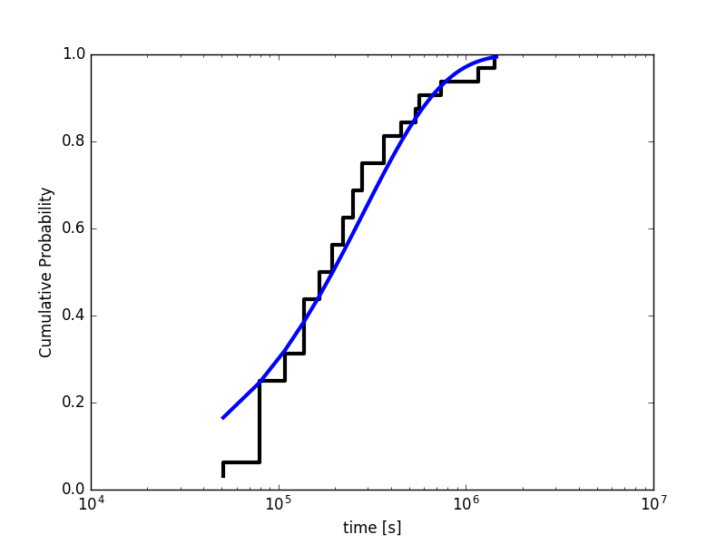
Figure Figure3 shows an example fit of the ECDF to the theoretical CDF for a Poisson process. To test the reliability of the fit, we can generate some data set according the theoretical CDF and perform a two-sample Kolmogorov-Smirnov (KS) test. The KS test provides the probability that the two sets of data are drawn from the same underlying distribution expressed in the so-called p-value. The null hypothesis is typically rejected for p-value < 0.05. The script cdf-analysis.py also performs the KS test and prints the p-value. What is the p-value we obtain from your dataset of transition times?
 1.8.17