 |
|
|
| |
|
|
Once this tutorial is completed students will learn to:
The tarball for this project contains the following folders:
Variationally enhanced sampling [117] is based on the the following functional of the bias potential:
\[ \Omega [V] = \frac{1}{\beta} \log \frac {\int d\mathbf{s} \, e^{-\beta \left[ F(\mathbf{s}) + V(\mathbf{s})\right]}} {\int d\mathbf{s} \, e^{-\beta F(\mathbf{s})}} + \int d\mathbf{s} \, p(\mathbf{s}) V(\mathbf{s}), \]
where \(\mathbf{s}\) are the CVs to be biased, \( p(\mathbf{s}) \) is a predefined probability distribution that we will refer to as the target distribution, and \( F(\mathbf{s}) \) is the free energy surface. This functional can be shown to be convex and to have a minimum at:
\[ V(\mathbf{s}) = -F(\mathbf{s})-{\frac {1}{\beta}} \log {p(\mathbf{s})}. \]
The last equation states that once that the functional \( \Omega [V] \) is minimized, the bias and the target distribution allow calculating the free energy. The target distribution \( p(\mathbf{s}) \) can be chosen at will and it is the distribution of the CVs once that \( \Omega [V] \) has been minimized.
The variational principle is put to practice by expanding \( V(\mathbf{s}) \) in some basis set:
\[ V(\mathbf{s}) = \sum\limits_{i} \alpha_i \, f_i(\mathbf{s}), \]
where \( f_i(\mathbf{s}) \) are the basis functions and the \(\boldsymbol\alpha \) are the coefficients in the expansion. We then need to find the \(\boldsymbol\alpha \) that minimize \( \Omega [V] \). In principle one could use any optimization algorithm. In practice the algorithm that has become the default choice for VES is the so-called averaged stochastic gradient descent algorithm [6]. In this algorithm the \(\boldsymbol\alpha \) are evolved iteratively according to:
\[ \boldsymbol\alpha^{(n+1)} = \boldsymbol\alpha^{(n)}-\mu \left[ \nabla\Omega(\bar{\boldsymbol\alpha}^{(n)})+ H(\bar{\boldsymbol\alpha}^{(n)})[\boldsymbol\alpha^{(n)}-\bar{\boldsymbol\alpha}^{(n)}] \right] \]
where \(\mu\) is the step size, \(\bar{\boldsymbol\alpha}^{(n)} \) is the running average of \(\boldsymbol\alpha^{(n)} \) at iteration \( n \), and \(\nabla\Omega(\bar{\boldsymbol\alpha}^{(n)}) \) and \(H(\bar{\boldsymbol\alpha}^{(n)}) \) are the gradient and Hessian of \( \Omega[V] \) evaluated at the running average at iteration \( n \), respectively. The behavior of the coefficients will become clear in the examples below.
We will consider the same system employed for the metadynamics tutorial.
For the first VES simulation we will revisit the problem of the ion pair dissociation but replacing the metadynamics bias with a VES bias. The bias potential will be constructed on the distance Na-Cl as done before. We will still use the upper wall used in the metadynamics tutorial to make the actual example as similar as possible to the previous one. We will then see that VES has a more natural way to deal with barriers. All files needed for this example can be found in the Example1 folder.
Every VES simulation has three key ingredients:
For the basis set we will choose Legendre polynomials defined in the interval [0.23,0.7] nm. Legendre polynomials are a good choice for non-periodic CVs. A rule of thumb for choosing the order of the expansion is that an expansion of order N can capture features of the FES of approximately L/N where L is the length of the interval. In this case, an order of 10 is able to capture features of the order of around 0.05 nm. We will see afterwards that the order of the expansion is not critical as long as we obtain good sampling at convergence. If this is the case, it is possible to obtain finer features of the FES through reweighting. The syntax for this basis set in Plumed is:
__FILL__ bf1: BF_LEGENDRE ...ORDER=10compulsory keyword The order of the basis function expansion.MINIMUM=0.23compulsory keyword The minimum of the interval on which the basis functions are defined.MAXIMUM=0.8 ...compulsory keyword The maximum of the interval on which the basis functions are defined.
We will use a uniform target distribution:
\[ p(\mathbf{s})= 1/C \]
with \( C \) a normalization constant. Once that \( \Omega [V] \) is minimized, the bias potential satisfies (up to an arbitrary constant):
\[ V(\mathbf{s}) = - F(\mathbf{s}) \]
This is the same relation that holds for non-tempered metadynamics.
The syntax for the bias potential in Plumed is:
__FILL__ td1: TD_UNIFORM b1: VES_LINEAR_EXPANSION ...ARG=d1the input for this action is the scalar output from one or more other actions.BASIS_FUNCTIONS=bf1compulsory keyword the label of the one dimensional basis functions that should be used.GRID_BINS=300the number of bins used for the grid.TARGET_DISTRIBUTION=td1 ...the label of the target distribution to be used.
Finally we have to choose the optimization algorithm. The standard is the averaged stochastic gradient descent. One has to define two parameters: the stride and the step size. The stride is the number of steps in which samples are collected to calculate the gradient and hessian of \( \Omega [V] \) and the step size is the step by which the coefficients are evolved at every optimization steps. Both of this parameters are connected. Increasing the stride will have an effect similar to reducing the step size. It has become traditional to choose a stride of around 500-2000 steps. It must be noted that we are not looking for an accurate estimation of the gradient, since for this we would need to sample all the CV space. The step size in the optimization has a strong connection with the height of typical barriers in the system. The larger the barriers, the larger the step size needed such that the bias can grow fast enough to overcome them. For this example we have chosen a stride of 500 steps and a step size of 0.5 kJ/mol. The syntax in Plumed is:
__FILL__ o1: OPT_AVERAGED_SGD ...BIAS=b1compulsory keyword the label of the VES bias to be optimizedSTRIDE=500compulsory keyword the frequency of updating the coefficients given in the number of MD steps.STEPSIZE=0.5compulsory keyword the step size used for the optimizationFES_OUTPUT=100how often the FES(s) should be written out to file.BIAS_OUTPUT=500how often the bias(es) should be written out to file.COEFFS_OUTPUT=10 ...compulsory keyword ( default=100 ) how often the coefficients should be written to file.
Now that we have set the scene, we can run our simulation using the run.sh script in the Example1 folder. The simulation will produce several files:
You can first observe how the system moves in the CV space in a fashion similar to metadynamics. Then we can see the evolution of \(\boldsymbol\alpha \) and \(\bar{\boldsymbol\alpha} \) . The first lines of the file coeffs.data are:
#! FIELDS idx_d1 b1.coeffs b1.aux_coeffs index
#! SET time 0.000000
#! SET iteration  0
#! SET type LinearBasisSet
#! SET ndimensions  1
#! SET ncoeffs_total  11
#! SET shape_d1  11
       0         0.0000000000000000e+00         0.0000000000000000e+00       0
       1         0.0000000000000000e+00         0.0000000000000000e+00       1
       2         0.0000000000000000e+00         0.0000000000000000e+00       2
       3         0.0000000000000000e+00         0.0000000000000000e+00       3
       4         0.0000000000000000e+00         0.0000000000000000e+00       4
       5         0.0000000000000000e+00         0.0000000000000000e+00       5
       6         0.0000000000000000e+00         0.0000000000000000e+00       6
       7         0.0000000000000000e+00         0.0000000000000000e+00       7
       8         0.0000000000000000e+00         0.0000000000000000e+00       8
       9         0.0000000000000000e+00         0.0000000000000000e+00       9
      10         0.0000000000000000e+00         0.0000000000000000e+00      10
#!-------------------


#! FIELDS idx_d1 b1.coeffs b1.aux_coeffs index
#! SET time 10.000000
#! SET iteration  10
#! SET type LinearBasisSet
#! SET ndimensions  1
#! SET ncoeffs_total  11
#! SET shape_d1  11
       0         0.0000000000000000e+00         0.0000000000000000e+00       0
       1         5.1165453234702052e-01         1.1482045941475065e+00       1
       2        -1.0356798763597277e+00        -1.7365051185667855e+00       2
       3        -5.1830527698835660e-01        -1.1651638070736938e+00       3
       4         4.1754103138162207e-01         4.8203393927719917e-01       4
       5         3.2087945211009694e-01         6.6606116920677805e-01       5
       6        -1.5499943980403830e-01        -4.7946750842365812e-03       6
       7        -1.1433825688016251e-01        -1.5099503286093419e-01       7
       8         9.8787914656136719e-02         1.3156529595420300e-02       8
       9         4.4467081175713474e-03        -8.7160339645570323e-02       9
      10        -1.1504176822089783e-01        -1.5789737594248379e-01      10
#!-------------------
The first column are the coefficient indices, the second are the \(\bar{\boldsymbol\alpha} \), and the third are the \(\boldsymbol\alpha \). Each block in the file corresponds to a different iteration, in this case iteration 0 and 10. We can plot the evolution of the coefficients using the gnuplot script plotCoeffs.gpi . The output should be similar to the next figure.
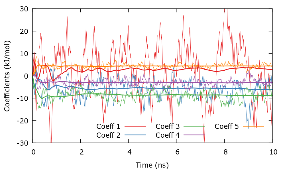
The \(\boldsymbol\alpha \) change fast and oscillate around some mean value. The \(\bar{\boldsymbol\alpha} \) evolve smoothly until they stabilize around some equilibrium value. It is important to remember that the bias is a function of \(\bar{\boldsymbol\alpha} \) and since these evolve smoothly, so will the bias. Once that the \(\bar{\boldsymbol\alpha} \) have stabilized, the simulation can be considered converged.
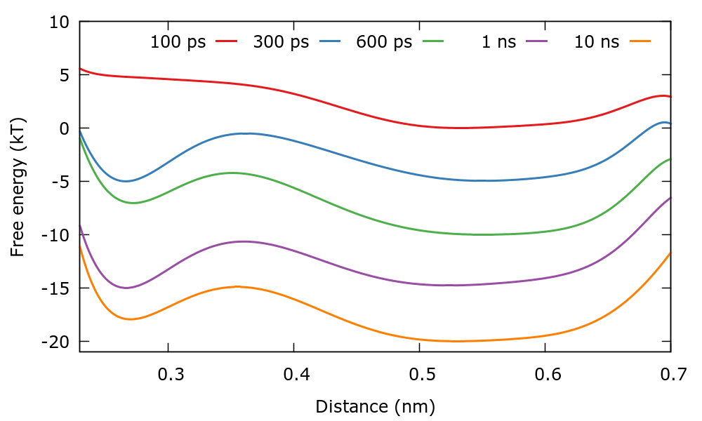
It is also interesting to observe how the estimation of the FES evolves in time. For this we will plot the FES using the files fes.b1.iter-<iteration-number>. There is a gnuplot script plotFes.gpi that you can use for this purpose. At variance with metadynamics, in this case there is no growing offset in the bias and therefore we will have to shift the FES ourselves to distinguish several FES at different times in the same plot.
We can also calculate the height of the barrier as we did in the metadynamics tutorial. The files for carrying out this task can be found in the Barrier_calculation folder. Remember that the accuracy of this calculation is limited by the fact that we have chosen a small order in the basis set expansion. We will discuss this aspect in greater detail in the next example.
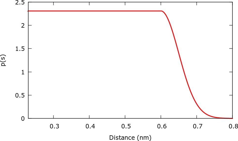
In this example we will consider other choices of target distributions and we will understand the influence of the order of the basis set expansion. The files needed for this example are contained in the directory Example2. Instead of introducing a barrier as done in the example above, in this case we will use a uniform target distribution in the interval [0.23:0.6] nm and decaying to zero in the interval [0.6:0.8] nm. The expression is:
MISSING EQUATION TO BE FIXED
where \( s_0=0.6\) nm and \( \sigma=0.05\). To define this \( p(s) \) in Plumed the input is:
__FILL__ td1: TD_UNIFORMMINIMA=0.23The minimum of the intervals where the target distribution is taken as uniform.MAXIMA=0.6The maximum of the intervals where the target distribution is taken as uniform.SIGMA_MAXIMA=0.05 b1: VES_LINEAR_EXPANSION ...The standard deviation parameters of the Gaussian switching functions for the maximum of the intervals.ARG=d1the input for this action is the scalar output from one or more other actions.BASIS_FUNCTIONS=bf1compulsory keyword the label of the one dimensional basis functions that should be used.TEMP=300.0the system temperature - this is needed if the MD code does not pass the temperature to PLUMED.GRID_BINS=300the number of bins used for the grid.TARGET_DISTRIBUTION=td1 ...the label of the target distribution to be used.
We will choose a basis set of order 20 to be able to capture the features of the FES with detail. If you are doing this example in a group, each member of the group can choose a different order in the expansion, for instance 5, 10, 20, and 40. The syntax in Plumed is:
__FILL__ bf1: BF_LEGENDRE ...ORDER=20compulsory keyword The order of the basis function expansion.MINIMUM=0.23compulsory keyword The minimum of the interval on which the basis functions are defined.MAXIMUM=0.8 ...compulsory keyword The maximum of the interval on which the basis functions are defined.
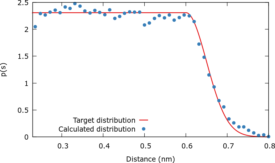
Once that you start running the simulation, a file named targetdist.b1.data will be created. This file contains the chosen target distribution. We can plot it to confirm that it is what we are looking for. There is a gnuplot script plotTargetDistrib.gpi that creates the following plot.
As the simulation runs, it is useful to control the evolution of the coefficients using the gnuplot script plotCoeffs.gpi.
The FES is calculated from the expression:
\[ F(\mathbf{s}) = -V(\mathbf{s})-{\frac {1}{\beta}} \log {p(\mathbf{s})} = \begin{cases} -V(s) \: & \mathrm{if} \: s<s_0 \\ -V(s) + \frac{(s-s_0)^2}{2\beta\sigma^2} \: & \mathrm{if} \: s>s_0\\ \end{cases} \]
In other words the bias potential is forced to create the upper barrier that we were explicitly introducing in the first example. When the FES is calculated the effect of the barrier is "subtracted" through \( p(s) \) and therefore the FES that we calculate does not include the barrier. This can be seen by plotting the fes.b1.iter-<iteration-number> files with gnuplot, for instance:
pl "./fes.b1.iter-10000.data" u 1:2 w l
This plot should be similar to the next figure.
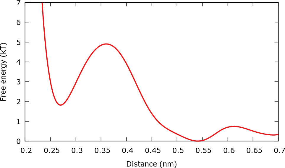
Only the interval [0.23:0.7] is plotted since there is little sampling in the region [0.7:0.8] due to the small value of \( p(s) \) in this region. As discussed before, if there is no sampling, it is not possible to obtain free energies.
When the simulation ends, it is interesting to check if in fact the sampled biased distribution is equal to the chosen target distribution. The scripts to calculate the sampled biased distribution are located in the directory BiasedDistribution. As usual, we will disregard the initial part of the simulation since in this period the bias is changing a lot. As done before, we get rid of the first 2 ns of simulation using sed:
sed '2,10000d' ../COLVAR > COLVAR
Once that the coefficients in the expansion have stabilized it is possible to calculate the biased distribution of CVs by constructing a histogram with equal weights for all points. This distribution should be equal to the target distribution \( p(s) \). The histogram can be calculated in plumed using the following input in the plumed.dat file:
__FILL__ distance: READFILE=COLVARcompulsory keyword the name of the file from which to read these quantitiesIGNORE_TIME( default=off ) ignore the time in the colvar file.VALUES=d1 hh1: HISTOGRAM ...compulsory keyword the values to read from the fileARG=distancethe input for this action is the scalar output from one or more other actions.GRID_MIN=0.2compulsory keyword the lower bounds for the gridGRID_MAX=0.8compulsory keyword the upper bounds for the gridGRID_BIN=100the number of bins for the gridBANDWIDTH=0.004 ... DUMPGRIDcompulsory keyword the bandwidths for kernel density estimationGRID=hh1compulsory keyword the action that creates the grid you would like to outputFILE=histocompulsory keyword ( default=density ) the file on which to write the grid.FMT=%24.16ethe format that should be used to output real numbers
and running (or using the run.sh script):
plumed --no-mpi driver --plumed plumed.dat --noatoms > plumed.out
The next plot shows that in fact the sampled distribution agrees with the target distribution.
Once that the coefficients are stabilized it is possible to reweight using the standard umbrella sampling formula [112] . In this case the weight assigned to each configuration is:
\[ w(\mathbf{R}) \propto e^{\beta V(\mathbf{s})}. \]
The files needed for this reweighting are contained in the folder ReweightDistance. The procedure to the the reweighting and plot the results is similar to the ones in the cases above and therefore it is not described in detail. The reweighted FES is plotted in the next figure and compared to the FES calculated from the formula \( V(\mathbf{s}) = -F(\mathbf{s})-{\frac {1}{\beta}} \log {p(\mathbf{s})} \).
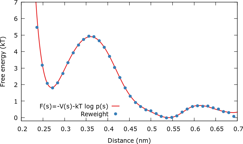
The two curves do not differ much since the order of the expansion was relatively large. What happens if you chose a lower or higher order in the expansion?
In this section we will restart the simulation that we have performed in our second example. In directory Example2, cd to the folder Restart. To restart the simulation we will need:
Therefore we execute in the command line the following commands:
cp ../restart .
cp ../COLVAR .
cp ../coeffs.data .
In order to restart, the RESTART keyword must be added at the beginning of the input file for PLUMED named plumed.restart.dat:
RESTART

d1:  DISTANCE ATOMS=319,320
.
.
.
Then the simulation can be restarted using the script runRestart.sh . Check that the output of the new simulation is appended to the COLVAR file, that the starting time of the new simulation is the ending time of the old simulation, that CV values are coherent, and that coefficients evolve continuously.
As an exercise, you can use a target distribution consisting in a gaussian centered at the dissociation barrier. The syntax in Plumed is:
__FILL__ td1: TD_GAUSSIANCENTER1=0.325The centers of the Gaussian distributions.SIGMA1=0.03 b1: VES_LINEAR_EXPANSION ...The standard deviations of the Gaussian distributions.ARG=d1the input for this action is the scalar output from one or more other actions.BASIS_FUNCTIONS=bf1compulsory keyword the label of the one dimensional basis functions that should be used.TEMP=300.0the system temperature - this is needed if the MD code does not pass the temperature to PLUMED.GRID_BINS=300the number of bins used for the grid.TARGET_DISTRIBUTION=td1 ...the label of the target distribution to be used.
Gaussian target distributions are useful to focus the sampling on a particular region of CV space. This has been used in protein folding problems to focus the sampling on the small but relevant folded state [102].
We suggest an exercise to gain experience in choosing the parameters of the optimization algorithm. The averaged stochastic gradient descent algorithm has two parameters: the stride and the step size. Normally a stride of around 500-2000 steps is used. However it is not always easy to choose the step size. Luckily, the algorithm is quite robust and will work for different step sizes.
Run different simulation using step sizes \( \mu = 0.001 \) and \( \mu = 10 \) and try to rationalize the behavior. Normally, when the step size is too large, the system gets stuck in CV space and coefficients oscillate wildly. When the step size is too small, the algorithm runs out of "steam" too fast and the simulation converges slowly. These two extreme cases should be avoided.
The purpose of this first tutorial was to introduce the student to VES. At this point one can see that VES is a powerful and versatile enhanced sampling method. We suggest to explore different possibilities of basis sets and target distributions. It is also interesting to experiment with different optimization algorithms and parameters of these.
The next tutorial will deal with the use of the well-tempered target distribution and the construction of biases on 2 CVs.
 1.8.17