 |
|
|
| |
|
|
In this Masterclass, we will discuss how to monitor and optimize the performances of a PLUMED-enhanced MD simulation.
Once you have completed this Masterclass you will be able to:
For this masterclass you will need versions of PLUMED and GROMACS that are compiled using the MPI library. Thus follow the instructions that are reported for PLUMED Masterclass 21.5: Simulations with multiple replicas.
Natively-compiled GROMACS and PLUMED will be significantly faster than the conda versions that we are providing. Since we are focusing on performance here, this might be the right time to learn how to install them on your own.
The data needed to execute the exercises of this Masterclass can be found on GitHub. You can clone this repository locally on your machine using the following command:
git clone https://github.com/plumed/masterclass-21-7.git
Notice that the results of these exercises might depend on the details of the hardware and software you are using. It is thus instructive to test them on different architectures, or with different PLUMED or GROMACS versions.
In these exercises you will have to maximise the performance of your simulation. When using GROMACS, the common way to report performances is to check at how many ns/day the simulation can produce. At the end of the log file you should find lines like these ones
               Core t (s)   Wall t (s)        (%)
       Time:      141.898       11.825     1200.0
                 (ns/day)    (hour/ns)
Performance:       14.628        1.641
Here, the higher the ns/day the faster your simulation will be. Another important information it the wallclock time, that indicates how many seconds elapsed since the start of your simulation. If you then run the same input file using PLUMED as well you will instead see something like this:
               Core t (s)   Wall t (s)        (%)
       Time:      170.519       14.210     1200.0
                 (ns/day)    (hour/ns)
Performance:       12.173        1.972
Finished mdrun on rank 0 Thu Apr 22 16:37:32 2021

PLUMED:                                               Cycles        Total      Average      Minimum      Maximum
PLUMED:                                                    1     2.009397     2.009397     2.009397     2.009397
PLUMED: 1 Prepare dependencies                          1001     0.004042     0.000004     0.000003     0.000013
PLUMED: 2 Sharing data                                  1001     0.151432     0.000151     0.000032     0.019904
PLUMED: 3 Waiting for data                              1001     0.021681     0.000022     0.000005     0.013026
PLUMED: 4 Calculating (forward loop)                    1001     1.392920     0.001392     0.000349     0.032230
PLUMED: 5 Applying (backward loop)                      1001     0.303819     0.000304     0.000089     0.025517
PLUMED: 6 Update                                        1001     0.003255     0.000003     0.000002     0.000175
Notice that:
Notice that the total time spent using PLUMED is approximately equal to the increment in the wallclock time. This might be different when using a GPU (and indeed the increment in the wallclock time should be smaller). This extra time measures the cost of using PLUMED. The goal of this Masterclass is to understand how to decrease this extra time without impacting the result of your simulation.
Notice that PLUMED gives a breakdown of the time spent. Some rows correspond to communication, and might become important if you run with a lot of MPI processes. Usually, most of the time is spent in the forward loop, where collective variables are calculated.
You can obtain a more detailed breakdown adding to your input this line:
DEBUG DETAILED_TIMERS( default=off ) switch on detailed timers
The tail of the log will then look like this:
PLUMED:                                               Cycles        Total      Average      Minimum      Maximum
PLUMED:                                                    1     2.055374     2.055374     2.055374     2.055374
PLUMED: 1 Prepare dependencies                          1001     0.004168     0.000004     0.000003     0.000023
PLUMED: 2 Sharing data                                  1001     0.118547     0.000118     0.000033     0.016011
PLUMED: 3 Waiting for data                              1001     0.008541     0.000009     0.000005     0.000035
PLUMED: 4 Calculating (forward loop)                    1001     1.449592     0.001448     0.000375     0.034236
PLUMED: 4A 0 @0                                         1001     0.004118     0.000004     0.000002     0.000134
PLUMED: 4A 4 d                                          1001     0.293253     0.000293     0.000011     0.023584
PLUMED: 4A 5 cn                                         1001     0.810816     0.000810     0.000308     0.034087
PLUMED: 4A 7 @7                                           11     0.000045     0.000004     0.000003     0.000008
PLUMED: 4A 8 @8                                         1001     0.225797     0.000226     0.000016     0.021056
PLUMED: 4A 9 @9                                         1001     0.066718     0.000067     0.000010     0.016033
PLUMED: 5 Applying (backward loop)                      1001     0.349111     0.000349     0.000120     0.025091
PLUMED: 5A 0 @9                                         1001     0.003697     0.000004     0.000003     0.000015
PLUMED: 5A 1 @8                                         1001     0.002814     0.000003     0.000002     0.000012
PLUMED: 5A 2 @7                                           11     0.000023     0.000002     0.000002     0.000002
PLUMED: 5A 4 cn                                         1001     0.102383     0.000102     0.000063     0.013438
PLUMED: 5A 5 d                                          1001     0.008055     0.000008     0.000006     0.000148
PLUMED: 5A 9 @0                                         1001     0.002417     0.000002     0.000002     0.000014
PLUMED: 5B Update forces                                1001     0.191250     0.000191     0.000020     0.023919
PLUMED: 6 Update                                        1001     0.003271     0.000003     0.000002     0.000166
Notice that for both the forward and the backward loop you are shown with a breakdown of the time required for each of the actions included in the input file. You should recognize the name of the actions that you defined, whereas unnamed actions are referred to with a generic @-number that corresponds to their position in the input file. From this detailed log you can also appreciate how often each action has been performed. PLUMED tries to optimize this, e.g., only computing variables when they are needed. This breakdown is very useful to know where you should direct your effort.
As a first test system we will consider a single Na Cl pair in a water box. The two ions are expected to attract each other, so that the bound conformation should be stable. The free energy as a function of the distance between the two ions should thus have a minimum followed by a barrier. At larger distances, it is not expected to become flat but rather to decrease as -2*kBT log d, due to the entropic contribution, and then to grow again when reaching the boundaries of the simulation box. In this exercise we will compute the free-energy as a function of the distance between the two ions. As collective variables we will use the distance between the two ions as well as the number of water oxygens that are coordinated with the sodium ion.
In the data/exercise1 folder of the GitHub repository of this Masterclass, you will find a topol.tpr file, which is needed to perform a MD simulation of this system with GROMACS. You can then create a plumed.dat file like this one as a starting point:
# vim:ft=plumed NA: GROUP ATOMSthe numerical indexes for the set of atoms in the group. =1 CL: GROUP ATOMSthe numerical indexes for the set of atoms in the group. =2 WAT: GROUP ATOMSthe numerical indexes for the set of atoms in the group. =3-8544:3 d: DISTANCE ATOMSthe pair of atom that we are calculating the distance between. =NA,CL cn: COORDINATION GROUPAFirst list of atoms. =1 GROUPBSecond list of atoms (if empty, N*(N-1)/2 pairs in GROUPA are counted). =WAT R_0 could not find this keyword =0.3 PRINT ARGthe input for this action is the scalar output from one or more other actions. =d,cn STRIDEcompulsory keyword ( default=1 ) the frequency with which the quantities of interest should be output =100 FILEthe name of the file on which to output these quantities =COLVAR METAD ARGthe input for this action is the scalar output from one or more other actions. =d,cn SIGMAcompulsory keyword the widths of the Gaussian hills =0.05,0.1 HEIGHTthe heights of the Gaussian hills. =0.1 PACEcompulsory keyword the frequency for hill addition =10 BIASFACTORuse well tempered metadynamics and use this bias factor. =5
As usual, you can run a simulation with the following command
gmx_mpi mdrun -plumed plumed.dat -nsteps 100000
For the first three points, you can run relatively short simulations, so choose nsteps based on what you can quickly test on your machine. For the fourth point instead you will need to reach convergence. A time on the order of a ns should be more the sufficient.
For this first point, we will focus on the calculation and update of the metadynamics bias. We will try to have a simulation that runs faster without changing significantly the result. Check the manual of METAD and find out how to speed up this calculation. A few hints:
Notice that these changes are not expected to impact the convergence of the algorithm. Thus, you do not need a converged simulation to measure the impact on performances.
For this second point, we will focus on the calculation of one of the two biased collective variables, namely the coordination of the Na ion with water oxygens. We will try to have a simulation that runs faster without changing significantly the result. Check the manual of COORDINATION and find out how to speed up this calculation. A few hints:
Notice that these changes are not expected to impact the convergence of the algorithm. Thus, you do not need a converged simulation to measure the impact on performances.
For this third point, we will try to make sure that GROMACS runs at its maximum speed. For this you will have to check GROMACS manual. A few hints:
-pin on option improves performances.Notice that these changes are not expected to impact the convergence of the algorithm. Thus, you do not need a converged simulation to measure the impact on performances.
We will now make modifications to the algorithm so as to be able to arrive to the same result running a shorter simulation. Try to play with METAD parameters and see if you can improve them. A few hints:
Notice that these changes are expected to impact the convergence of the algorithm. Thus, you do not need a converged simulation to measure the impact on performances, and you have to make sure that the statistical accuracy is comparable.
As a final step, analyze the simulations performed so far to compute the standard binding free energy between the two species. Notice that even though this is defined at 1M concentration, the calculations that you are running are actually at infinite dilution.
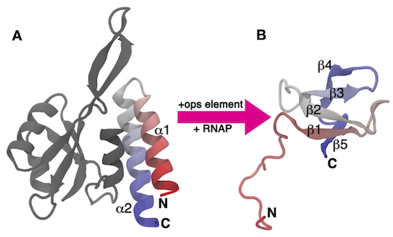
In this exercise, we will work with the C-terminal domain (CTD) of the RfaH virulence factor from Escherichia coli introduced in PLUMED Masterclass 21.4: Metadynamics (see Exercise 6: A 'real-life' application). This part of the system, which we refer to as RfaH-CTD, undergoes a dramatic conformational transformation from β-barrel to α-helical, which is stabilized by the N-terminal domain of the RfaH virulence factor (see Fig. masterclass-21-7-RfaH-CTD-fig).
RfaH-CTD is simulated using a simplified, structure-based potential, called SMOG. The SMOG energy function has been designed to have two local minima corresponding to the β-barrel and α-helical states of RfaH-CTD. To achieve this goal, the SMOG energy function promotes native contacts, i.e. interactions that are present in the native structure(s). When using structure-based force fields, a function of the coordinates that is correlated with the energy of the system, such as the total number of native contacts, has been shown to be a good CV for enhanced-sampling simulations. Unfortunately, these types of CVs often involve a large number of atoms and are therefore computationally expensive to calculate at every step of the simulation. In this exercise, we will learn how to write and optimize these types of CVs.
In the data/exercise2 folder of the GitHub repository of this Masterclass, you will find:
stateA.pdb) and α-helical (stateB.pdb) states;topol.tpr file, which is needed to perform a MD simulation of this system with GROMACS;plumed.dat) to perform a metadynamics simulation using the total number of native contacts as CV. These contacts are defined using only the β-barrel conformation, which is the most populated state in the conditions we are simulating.The provided PLUMED input file looks as follows:
# reconstruct molecule WHOLEMOLECULES ENTITY0the atoms that make up a molecule that you wish to align. =1-330 # CA-RMSDs from the two reference conformations # useful for monitoring the distance from the two metastable states rmsd_A: RMSD REFERENCEcompulsory keyword a file in pdb format containing the reference structure and the atoms involved in the CV. =stateA.pdb TYPEcompulsory keyword ( default=SIMPLE ) the manner in which RMSD alignment is performed. =OPTIMAL NOPBC( default=off ) ignore the periodic boundary conditions when calculating distances rmsd_B: RMSD REFERENCEcompulsory keyword a file in pdb format containing the reference structure and the atoms involved in the CV. =stateB.pdb TYPEcompulsory keyword ( default=SIMPLE ) the manner in which RMSD alignment is performed. =OPTIMAL NOPBC( default=off ) ignore the periodic boundary conditions when calculating distances # list of 379 distances between atoms that are closer # than 0.6 nm in the reference PDB file (stateA.pdb, β-barrel state) d1: DISTANCE ATOMSthe pair of atom that we are calculating the distance between. =1,110 NOPBC( default=off ) ignore the periodic boundary conditions when calculating distances d2: DISTANCE ATOMSthe pair of atom that we are calculating the distance between. =1,115 NOPBC( default=off ) ignore the periodic boundary conditions when calculating distances # __FILL__ d379: DISTANCE ATOMSthe pair of atom that we are calculating the distance between. =239,265 NOPBC( default=off ) ignore the periodic boundary conditions when calculating distances # list of 379 switching functions to define a contact from the distance between two atoms c1: CUSTOM FUNCcompulsory keyword the function you wish to evaluate =1-erf(x^4) ARGthe input for this action is the scalar output from one or more other actions. =d1 PERIODICcompulsory keyword if the output of your function is periodic then you should specify the periodicity of the function. =NO c2: CUSTOM FUNCcompulsory keyword the function you wish to evaluate =1-erf(x^4) ARGthe input for this action is the scalar output from one or more other actions. =d2 PERIODICcompulsory keyword if the output of your function is periodic then you should specify the periodicity of the function. =NO # __FILL__ c379: CUSTOM FUNCcompulsory keyword the function you wish to evaluate =1-erf(x^4) ARGthe input for this action is the scalar output from one or more other actions. =d379 PERIODICcompulsory keyword if the output of your function is periodic then you should specify the periodicity of the function. =NO # sum of switching functions = total number of contacts cv: COMBINE ARGthe input for this action is the scalar output from one or more other actions. =c1,c2,c3,c4,c5,c6,c7,c8,c9,c10,c11,c12,c13,c14,c15,c16,c17,c18,c19,c20,c21,c22,c23,c24,c25,c26,c27,c28,c29,c30,c31,c32,c33,c34,c35,c36,c37,c38,c39,c40,c41,c42,c43,c44,c45,c46,c47,c48,c49,c50,c51,c52,c53,c54,c55,c56,c57,c58,c59,c60,c61,c62,c63,c64,c65,c66,c67,c68,c69,c70,c71,c72,c73,c74,c75,c76,c77,c78,c79,c80,c81,c82,c83,c84,c85,c86,c87,c88,c89,c90,c91,c92,c93,c94,c95,c96,c97,c98,c99,c100,c101,c102,c103,c104,c105,c106,c107,c108,c109,c110,c111,c112,c113,c114,c115,c116,c117,c118,c119,c120,c121,c122,c123,c124,c125,c126,c127,c128,c129,c130,c131,c132,c133,c134,c135,c136,c137,c138,c139,c140,c141,c142,c143,c144,c145,c146,c147,c148,c149,c150,c151,c152,c153,c154,c155,c156,c157,c158,c159,c160,c161,c162,c163,c164,c165,c166,c167,c168,c169,c170,c171,c172,c173,c174,c175,c176,c177,c178,c179,c180,c181,c182,c183,c184,c185,c186,c187,c188,c189,c190,c191,c192,c193,c194,c195,c196,c197,c198,c199,c200,c201,c202,c203,c204,c205,c206,c207,c208,c209,c210,c211,c212,c213,c214,c215,c216,c217,c218,c219,c220,c221,c222,c223,c224,c225,c226,c227,c228,c229,c230,c231,c232,c233,c234,c235,c236,c237,c238,c239,c240,c241,c242,c243,c244,c245,c246,c247,c248,c249,c250,c251,c252,c253,c254,c255,c256,c257,c258,c259,c260,c261,c262,c263,c264,c265,c266,c267,c268,c269,c270,c271,c272,c273,c274,c275,c276,c277,c278,c279,c280,c281,c282,c283,c284,c285,c286,c287,c288,c289,c290,c291,c292,c293,c294,c295,c296,c297,c298,c299,c300,c301,c302,c303,c304,c305,c306,c307,c308,c309,c310,c311,c312,c313,c314,c315,c316,c317,c318,c319,c320,c321,c322,c323,c324,c325,c326,c327,c328,c329,c330,c331,c332,c333,c334,c335,c336,c337,c338,c339,c340,c341,c342,c343,c344,c345,c346,c347,c348,c349,c350,c351,c352,c353,c354,c355,c356,c357,c358,c359,c360,c361,c362,c363,c364,c365,c366,c367,c368,c369,c370,c371,c372,c373,c374,c375,c376,c377,c378,c379 PERIODICcompulsory keyword if the output of your function is periodic then you should specify the periodicity of the function. =NO # metadynamics using "cv" metad: METAD ARGthe input for this action is the scalar output from one or more other actions. =cv # Deposit a Gaussian every 500 time steps, with initial height # equal to 1.2 kJ/mol and bias factor equal to 60 PACEcompulsory keyword the frequency for hill addition =500 HEIGHTthe heights of the Gaussian hills. =1.2 BIASFACTORuse well tempered metadynamics and use this bias factor. =60 # Gaussian width (sigma) based on the CV fluctuations in unbiased run SIGMAcompulsory keyword the widths of the Gaussian hills =10.0 # Gaussians will be written to file FILEcompulsory keyword ( default=HILLS ) a file in which the list of added hills is stored =HILLS ... # print useful stuff PRINT ARGthe input for this action is the scalar output from one or more other actions. =cv,rmsd_A,rmsd_B,metad.bias STRIDEcompulsory keyword ( default=1 ) the frequency with which the quantities of interest should be output =500 FILEthe name of the file on which to output these quantities =COLVAR
The objectives of this exercise are to:
Suggestions:
STRIDE option on the METAD line.Please keep in mind that:
gmx mdrun -plumed plumed.dat -ntomp 4 -noddcheck. You can adjust the number of CPU cores you want to use (here 4, OpenMP parallelization), based on the available resources. The system is not particularly big, therefore using a large number of cores might be inefficient.  1.8.17