 |
|
|
| |
|
|
The purpose of this Masterclass is to understand and test Funnel-Metadynamics (FM) in the study of a binding event for a paradigmatic model with PLUMED.
Once this Masterclass is completed, users will be able to:
In order to easily follow this masterclass, users should be able to:
Most of the required information can be found in PLUMED Masterclass 21.1: PLUMED syntax and analysis and PLUMED Masterclass 21.4: Metadynamics.
Unveiling the binding mechanism of a ligand to its molecular target is an important information to perform a successful drug design campaign. PLUMED allows to accurately compute binding free energies, thus allowing us to thoroughly identify the lowest energy ligand binding modes and binding pathways. The FM is a variant of Metadynamics, which enhances the sampling of ligand binding/unbinding towards its molecular target through the use of a funnel-shaped restraint. The latter is constructed as an external potential that limits the sampling of the ligand to the binding pocket and a slim region in the solvent, accelerating convergence and avoiding wasting time in sampling useless unbound states. In the following, we will learn how to use PLUMED to perform a FM simulation following the FM Advanced Protocol (FMAP) [118]. Below it is reported a recap of the basic metadynamics theory.
In metadynamics, an external history-dependent bias potential is constructed in the space of a few selected degrees of freedom \( \vec{s}({q})\), generally called collective variables (CVs) [80]. This potential is built as a sum of Gaussian kernels deposited along the trajectory in the CVs space:
\[ V(\vec{s},t) = \sum_{ k \tau < t} W(k \tau) \exp\left( -\sum_{i=1}^{d} \frac{(s_i-s_i({q}(k \tau)))^2}{2\sigma_i^2} \right). \]
where \( \tau \) is the Gaussian deposition stride, \( \sigma_i \) the width of the Gaussian for the \(i\)th CV, and \( W(k \tau) \) the height of the Gaussian. The effect of the metadynamics bias potential is to push the system away from local minima into visiting new regions of the phase space. Furthermore, in the long time limit, the bias potential converges to minus the free energy as a function of the CVs:
\[ V(\vec{s},t\rightarrow \infty) = -F(\vec{s}) + C. \]
In standard metadynamics, Gaussian kernels of constant height are added for the entire course of a simulation. As a result, the system is eventually pushed to explore high free-energy regions and the estimate of the free energy calculated from the bias potential oscillates around the real value. In well-tempered metadynamics [11], the height of the Gaussian is decreased with simulation time according to:
\[ W (k \tau ) = W_0 \exp \left( -\frac{V(\vec{s}({q}(k \tau)),k \tau)}{k_B\Delta T} \right ), \]
where \( W_0 \) is an initial Gaussian height, \( \Delta T \) an input parameter with the dimension of a temperature, and \( k_B \) the Boltzmann constant. With this rescaling of the Gaussian height, the bias potential smoothly converges in the long time limit, but it does not fully compensate the underlying free energy:
\[ V(\vec{s},t\rightarrow \infty) = -\frac{\Delta T}{T+\Delta T}F(\vec{s}) + C. \]
where \( T \) is the temperature of the system. In the long time limit, the CVs thus sample an ensemble at a temperature \( T+\Delta T \) which is higher than the system temperature \( T \). The parameter \( \Delta T \) can be chosen to regulate the extent of free-energy exploration: \( \Delta T = 0\) corresponds to standard MD, \( \Delta T \rightarrow\infty\) to standard metadynamics. In well-tempered metadynamics literature and in PLUMED, you will often encounter the term "bias factor" which is the ratio between the temperature of the CVs ( \( T+\Delta T \)) and the system temperature ( \( T \)):
\[ \gamma = \frac{T+\Delta T}{T}. \]
The bias factor should thus be carefully chosen in order for the relevant free-energy barriers to be crossed efficiently in the time scale of the simulation. Additional information can be found in the several review papers on metadynamics [79] [12] [128] [31]. To learn more: Summary of theory
The users can refer to the procedure introduced in PLUMED Masterclass 21.1: PLUMED syntax and analysis and PLUMED Masterclass 21.3: Umbrella sampling to install the required software. It is suggested that an optimized version of GROMACS is properly installed since the exercises will also require a simulation as input. Please remember to activate the module for the FM as reported here.
Please also install a working version of VMD that will be used together with two graphical user interfaces (GUIs) to create the PLUMED input file and analyse the results during the exercises. More information to download and install VMD can be found here.
The GUIs require the tcl tooltip library, which is not implemented in the software. You can download the library from its github repository. You should also download the GUIs themselves, which can be found in the folder funnel_gui in their github repository. No further installation is necessary, but in order to source the GUI the following command must always precede:
source /place/where/you/downloaded/tooltip.tcl
Therefore, an example on how to open the GUI to set up a FM simulation (e.g., funnel.tcl) would be to write the following lines in the VMD Tk console:
source /folder/where/you/downloaded/tooltip.tcl
source /folder/where/you/downloaded/funnel.tcl
During this masterclass, a request to source a GUI (funnel.tcl or ffs.tcl) will always translate to the above commands. You can find a detailed version of the procedure in the FMAP protocol paper [118].
The data needed to conduct the exercise shoulb be generated with VMD and a molecular dynamics engine. In case of problems in generating the requested data, an example can be found in Zenodo. Inside you will find:
FMAP_procedure.pdf: a pdf resuming all the steps in FMAP;README.md: a file containing general information about installation and setup;Supplementary_data_2: a folder containing example data for the exercises.In details, the latter includes:
2D-distance.dat: an example of a 2D free-energy surface (FES);BFES: a folder containing 80 files representing the 1D FES with respect to time (1 FES per 10 ns);COLVAR: an example of output file form the FM simulation;driver.dat: an example of input file for driver;fes_lr.dat: an example of low resolution FES;HILLS_800ns: an example of output file for a 800 ns FM run;plumed.dat: an example of PLUMED input file for a FM simulation;start.pdb: an example of coordinates file for the FM simulation;trj.trr: a strided version of a trajectory obtained through FM simulation.However, we strongly suggest to create new data in order to experience first-hand all protocol's steps.
All the compulsory files for the system of interest can be found in a dedicated repository:
git clone https://github.com/h2nch2co2h/masterclass-22-1
This repositoy contains 2 folders:
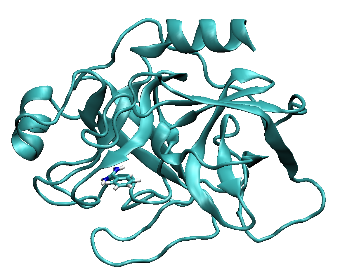
data: GROMACS input files, topologies, and index file for the system that we are going to simulate;slides: the presentation of the FM theory presented during the first lesson. We will simulate a paradigmatic system generally used to test and benchmark new binding free-energy approaches, the benzamidine-trypsin system (see Fig. masterclass-22-1-system.png). Although benzamidine is one of the simplest small molecules you could find in the ligand-target binding world, this system represents a good compromise between user-friendliness and biological importance. The binding happens in a very well-known pocket of trypsin, which has been thoroughly outlined by several X-ray structures. The amidine group in benzamidine is positively charged in physiological conditions and interacts with a negatively charged residue in the pocket (i.e., ASP171). In this masterclass we will try to analyse the binding/unbinding events between these two partners, with a particular focus in the estimate of the binding free energy. Additional information about convergence checks and the study of the saddle points in the lowest binding pathway will also be provided.
As first exercise, we will generate a PLUMED input file that could be used to run a FM simulation. For this purpouse, we will need a starting structure of the system under study that will be used to set up the funnel-shaped potential. As a general advice, this structure should be the output of the equilibration step (i.e., with the system brought at the correct simulation parameters and ready for the production run). For this exercise, the structure has been provided in the masterclass github (start.gro). Open VMD and source the first GUI (funnel.tcl) as explained in Setting up the software. Load the structure of the system and, when the simulation box will be visualised, call the interface by using the following command in the Tk console of VMD:
funnel_tk
This should open the interface and display a tentative orange funnel in VMD masterclass-22-1-funnel. The user is now able to customise the funnel with respect to the benzamidine-trypsin system.

An accurate description of all the steps to set up the funnel can be found in the Nature Protocols paper raniolo2020ligand. Here, we will briefly discuss the compulsory points for the simulation to start.
Hint for the user: in VMD all values are reported in Angstrom, whereas PLUMED works in nm. The conversion should be taken into account by the interface but always be careful about possible inconsistencies.
The first thing to correct is the orientation of the funnel, which can be done by selecting atoms in VMD or by changing the Cartesian coordinates of the points A and B that create the funnel. You can find these values in the boxes in the upper part of the interface, whereas the option to assign A or B to an atom can be activated through the switches directly below. For the sake of this exercise, the provided structure already has the ligand in the binding pocket, which will ease the setup process. However, this knowledge might be missing in other systems, thus requiring preceding docking calculations or an extensive scanning of the protein surface with FM.
Hint for the user: hovering over the options in the interface should display a small text explaining what each one does.
By visualizing the protein as new cartoon and the ligand (resname MOL) as licorice, it is possible to clearly see the binding pocket. Try to provide an acceptable orientation for the funnel, with the conical section faced towards the protein and the cylindrical one describing a possible unbindng route for benzamidine (see Fig. masterclass-22-1-funnel).
Hint for the user: choosing to assign points A and B by picking atoms is the fastest choice, just remember to press r after the selection to deactivate the pick mode.
At this point we only corrected the direction, so we should adapt all the other parameters to adjust the cone/cylinder ratios and depth. This is done through the following options:
Zcc: switching point between cone and cylinder, value 0 for Zcc corresponds to point A;Alpha: angle defining the width of the cone;RCyl: radius of the cylinder.Select a set of parameters that allow for benzamidine to explore the binding pocket (inside the conical section of the funnel) and unbind without colliding with the protein on the way out (inside the cylindrical part). A good choice in positions of points A and B and in parameters will allow for a swift convergence without possible artefacts in the simulation. Overall, the funnel-shaped restraint must cover completely the entrance of the binding pocket, including the residues at the edge since they can have a recruiting effect for the ligand. During the sampling the ligand will be simplified to its center of mass and will explore all the allowed volume. This should be considered for relatively big ligands, since covering large areas with the funnel might mean the loss of simulation time in exploring states that are not interesting in the binding process. For the current exercise, try not to have the funnel covering pure-solvent sections of the box and be as strict as possible to the binding site.
Once the funnel has been finalised, a few other parameters must be specified in order for the FM simulation to start. The funnel potential will be constructed as a grid file, so we need to provide dimensions to delimit it. This dimensions are defined by the following parameters:
Min fps.lp: minimum value along the funnel axis (taking point A as the 0);Max fps.lp: maximum value along the funnel axis (taking point A as the 0).At this point a bit of history. In the first version of FM, the dimensions of the grid were called linepos and linedist, which stands for the position on the funnel axis and distance from it, respectively. They have been transformed in fps.lp and fps.ld, with fps that stands for funnel positioning system. Limits for ld must not be specified since the minimum is 0 by definition and the maximum is computed based on the other parameters that have been provided (i.e., Alpha and min fps.lp).
Hint for the user: Min fps.lp can take either positive or negative values. For example if point A has been positioned deep in the bulk of the protein, positive values might be advisable since the ligand will never be able to pierce the protein. As for max fps.lp, the ligand should be able to sample portions of the solvent outside of the influence of the protein (e.g., the cutoff in the case of simulations). Since the solvent is sampled in the cylindrical part of the funnel, around 3-4 Angstroms of fps.lp should be assigned for the solvent sampling, outside of the protein electrostatic and vdw cutoffs.
With the edges of the grid decided, two walls are applied to enforce the sampling in the allowed region. This is necessary because if the center of mass of the ligand goes out of grid for any reason, the algorithm will output an error and the entire FM simulation will crash. For this reason, you can find the Low. wall and Up. wall parameters in the interface that should be set leaving 2-3 Angstroms from the grid edges. For example, with Min fps.lp and Max fps.lp of 0 and 40, a Low. wall of 2 and an Up. wall of 38 might be a good compromise.
After all the previous steps have been completed, make sure that the value at the right of ID is the same index as the structure that you used to set up the funnel, write in the box at the right of Ligand the atoms that should be recognised as part of the ligand in the VMD syntax and press enter. For example:
resname MOL
will consider all atoms of the residue called MOL (which in this case are all atoms of benzamidine).
resname MOL and noh
will instead select only the heavy atoms of residue MOL.
When ready, click on Apply and a PLUMED input file should be generated with all required options. You can print it to a file through the export feature. Please, check that all values have been correctly trasformed in the measurement unit accepted by PLUMED.
The newly created file contains all the compulsory lines to run a FM simulation. Few commands like WHOLEMOLECULES and RESTART can also be commented and will be discussed in the next exercise. Others must be completed by the user either with the interface, a text editor, or by hand in the VMD canvas. Here, we will briefly describe the missing parameters for the funnel, leaving to the user the job to complete the rest (i.e., METAD, LOWER_WALLS, and UPPER_WALLS).
REFERENCE: requires the name of the file that will be used to align the funnel to the protein during the simulation. Save the current system as a pdb and provide here the name of the pdb;ANCHOR: a protein atom that is close to the ligand along the supposed binding pathway. This is necessary in some cases to avoid periodic boundary conditions (PBC) problems and should be interactively chosen as previously done for point A and B;KAPPA: potential constant to generate the funnel-shaped restraint, requires a number in kJ/mol/nm^2 (for benzamidine around 35000 is fine).Hint for the user: the drop-down menu contains all parameters that require an entry in order to work. Depending on the option, VMD selections or numbers should be supplied. Please remember to always press enter after selecting an option and providing the wanted value. If you changed anything, please remember to export again the input file. The user is now free to customise his/her input. Be aware that modifications done by hand on the canvas will be overwritten upon pressing Apply.
This concludes the first exercise.
In this exercise we will finally run the FM simulation (applause noises). But before that, all necessary lines in the PLUMED input file created in Exercise 1: FM input generation must be completed. We remember that FM rely upon metadynamics to work, therefore the description of collective variables (CV) and all the necessary knownledge to set up a well-tempered Metadynamics are given for granted. The user can still refresh his/her memory with PLUMED Masterclass 21.4: Metadynamics. Suffice to say that in this case a distance between protein and ligand or fps.lp itself could be used as an argument for METAD.
The file runme.tpr has already been prepared for you to run and we will imply that the file from exercise 1 has been called plumed.dat. All you need to do is execute the following command:
gmx mdrun -s runme.tpr -deffnm firstFM -nsteps 125000000 -plumed plumed.dat
This represents 250 ns of FM simulation, which is unlikely to finish with a single-task launch. The objective of the exercise is not to reach convergence, but, depending from the computational resource at one disposal, an MPI job could achieve better results:
mpirun -np X gmx mdrun -s runme.tpr -deffnm firstFM -nsteps 125000000 -plumed plumed.dat
We also remember that gpu could be called with the -gpu_id flag and proper resource management can be controlle with the various -ntomp, -ntmpi, etc. For maximum performances, we would like to mention that FM supports WALKERS_MPI (the flag should be added both in METAD and FUNNEL in order for it to work).
Hint for the user: please remember that to use multiple walkers, the BIAS file, where the funnel potential is stored, and the HILLS file should be placed in the parent folder of the walkers by setting FILE=../BIAS and FILE=../HILLS as per last policy of GROMACS at this juncture. Please also be aware that several GB of files will be created, so avoid running such a calculation on a laptop.
Similarly to what has been seen for standard metadynamics, we can check the simulation through the following command:
plumed sum_hills --hills HILLS --stride 500 --mintozero
This should generate a free-energy surface (FES) file each 0.5 ns of simulation and comparing them with respect to time we can easily note if the profile does not change considerably. This is by no means a clear indication of convergence but it is one of the many checks that can be carried out to understand when to stop the simulation. Theoretically, depending also on the metadynamics parameters, 200 ns might not be enough to obtain full convergence, but could still be used for the post-processing phase.
At this point the user should just wait for the simulation to finish or to gather as much statistics as possible. During the simulation, the FM might crash giving an out of grid error. This is caused by the ligand jumping to a periodic image and thus abruptly leaving the grid representing the funnel potential. Two main scenario could happen:
Hint for the user: an imperfect setup of FM can drastically decrease the performance of the simulation. However, FM can be as fast as a standard Metadynamics with the correct precautions. One of the biggest time sinks is the alignment repeated for each simulation step to ensure the correct funnel placement with respect to a rotating and translating protein. If a full pdb is provided in REFERENCE, computing the roto-translational matrix will become a heavy task. We suggest to limit the number of atoms used to only CA atoms of structured portions of the protein. The user is encouraged to try and run few thousand steps (-nsteps flag) with different pdb files to see the difference in performance.
Regardless of convergence and time simulated, congratulations! You run your first FM simulation.
With the production run terminated, we can focus on analysis to check for convergence and compute the binding free energy for the benzamidine- trypsin complex. Firstly, we will repeat the same analysis done in exercise 2 but with the VMD interface (see Fig. masterclass-22-1-ffs.png). Please open VMD and source the second GUI called ffs.tcl. To display the interface you can write in the Tk console of VMD the command:
ffs_tk
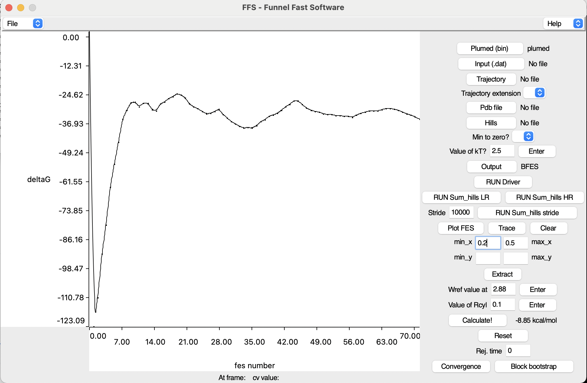
The user can immediately see that all options are on the right of the interface and most of the space is occupied by the central canvas that is used to plot graphs. As previously said, let's try generating FES files starting from the HILLS file created during the production run. For a sum_hills calculation, compulsory parameters are:
Output button and the last thing to do is to press RUN sum_hills LR or RUN sum_hills HR, depending on the required resolution of the FES file (low or high resolution, respectively). This would produce a single FES file that takes into account the entire simulation time.Our objective though is to check the differences of the FES with respect to time. Therefore, we can provide a stride value to print the FES every n steps and click on RUN Sum_hills stride. The process might take some time to complete, so wait for VMD to finish all calculations.
Hint for the user: the log of each job (e.g., RUN Sum_hills LR, RUN Sum_hills HR, and RUN Sum_hills stride) will be written in the Tk console of VMD. From there, the user can check that everything went smoothly.
By pressing Plot FES, one of the generated FES can be plotted in the VMD canvas. Depending on the graph resolution, the time requested to visualise it might change and up to 3D plots can be represented (the third dimension being transformed into a chromatic scale).
Each and every FES can provide a value for the binding free energy with respect to time and we can calculate the difference in binding free energy with the following formula:
\[ \Delta G_b = -1/\beta ln(C_0 \pi r_{cyl}^2) \int_{bound} e^{-\beta(W(z)-W_{ref})} dz, \]
with C0 being the standard concentration of 1 M for all reacting molecules, \( \beta \) the inverse of the Boltzmann constant multiplied by the temperature in Kelvin, W(z) the value of the potential mean force (PMF) in the bound poses, and Wref the PMF in the unbound region.
If you used fps.lp as your CV of selection for metadynamics then you are set. Otherwise, the user is requested to reweight with respect to it and create again the FES files in function of fps.lp. Instructions on how to reweight on an auxiliary CV can be found in PLUMED Masterclass 21.4: Metadynamics. This step is necessary because the entropic correction contained in the above formula considers the variable of intergration as the position along the funnel.
Hint for the user: if you reweighted your simulation, make sure that the created files have the same name as the files generated by sum_hills (e.g., fes_1.dat). The interface automatically takes all the files with that format and will not recognise any other FES file.
Before, the user had to create his/her own script to compute the bindng free energy, now though the value is provided by clicking on Calculate!. The bound interval W(z) can be defined by using the min_x and max_x boxes, whereas the reference value Wref for the unbound must be written in the corresponding box. The user should try to compute a free energy from a FES of choice picking the intervals more appropriate to the results obtained from the production run. The estimate will apper at the right of the button, already rescaled in kcal/mol and taking into consideration the entropic correction coming from the presence of the funnel. Repeating this analysis for different simualtion times will give the behaviour of the binding free energy with respect to time, which is an additional check to verify convergence of the simulation. In particular, a converged simulation should present a stable value for the free energy with the progress of time. This can be done by pressing the Convergence button, which will take all the fes files generated by sum_hills in the working directory (spedified by the Output option). Upon clicking, the user should see the new plot of the free energy in function of time. Moreover, the user can find the average-on-the-fly and the standard deviation of the computation in the VMD TK console.
Hint for the user: the calculation of the binding free energy with respect to time is initially done taking the whole dataset, however the first steps in metadynamics are generally discarded from statistical measurements. This can be done by specifying a value for the reject time in units of FES stride numbers. Therefore if you generated one FES per ns of simulation, the first 100 ns in a 800 ns production run can be erased by putting 100 on the box at the right of Rej. time. This will most likely reduce the error of the calculation and provide a more accurate estimate.
As a further instrument to check convergence, the interface incorporates a block bootstrap analysis. This approach takes the same interval considered for the calculation of the average-on-the-fly and standard deviation, but divides the remaining dataset in 10 blocks. Each of them will be subjected to a bootstrap analysis, obtaining in the end the mean and standard error for each block (visible in the Tk console) and a visual representation of how the distribution of values behaves in the block. For converged simulations, averages of the last blocks should be very similar and their distribution should resemble a normal distribution. Deviation from this behaviour might indicate missing convergence.
The user is encouraged to try different reject times with both the convergence tool and the block bootstrap analysis.
Hint for the user: this analysis might not be possible if you could not simulate a statistically-relevant amount of time. In fact, the approach requires a minimum of 500 points in total (50 per block) and will stop otherwise. This problem can be circumvented by reducing the stride in the generation of the FES, but this workaround is advised against since there would not be much difference among FES files not due to convergence but because the system would not have enough time to evolve. The user can use the 800 FES that have been prepared on Zenodo as a substitution.
Another analysis that can be done to check convergence in a binding free-energy calculation is to plot the sampling of the selected CVs with respect to time to see if the ligand was able to bind/unbind a number of times, thus gathering sufficient statistics on the binding process. This can be achieved by plotting with a software of choice the columns of time and collective variable (CV) used for the FM simulation (e.g., gnuplot, xmgrace, matplotlib, etc.).
Hint for the user: using multiple walkers, it is possible to experience a compartmentalization effect, each walker exploring only a subset of the whole CV space. To check if the potential has been correctly placed, the user can launch a single walker loading all the bias that has been added and should observe the binding/unbinding in a relatively low number of steps.
We will finish this exercise with two more interactive features of the interface. Up to now, we only spoke about graphs and distributions, but the user should always observe what happened in the simulation box. For this reason, please process your production run aligning the protein at the center of the box, displaying only benzamidine and trypsin (group Complex in the index file complex.ndx), and striding the simulation so as to have around 100 frames. This can be done through the trjconv function of GROMACS and the use of the flags -pbc and -fit.
Example:
gmx_mpi trjconv -f simulation.xtc -n complex.ndx -s runme.tpr -pbc nojump -o sim_nojump.xtc -dt 10000
gmx_mpi trjconv -f sim_nojump.xtc -n complex.ndx -s runme.tpr -fit rot+trans -o sim_aligned.xtc
The user can employ a combination of his/her own choice, it will just help in visualising the structures in VMD. The newly created trajectory can be loaded in VMD together with a coordinate file through the New Molecule and Load Data into Molecule options in File. Once this is done, we can track the state of each frame in the FES. For this, we will need one of the FES generated in the previous steps and a COLVAR file that has a number of lines equal to the frames in the loaded simulation. This job can be achieved by using the driver functionality of PLUMED either by hand or through the interface. Since the former is given for granted, we will proceed following the latter. The compulsory options to run a driver calculation on the interface are:
As always the output shall be saved in the folder specified by Output and when everything is ready you can just press RUN Driver. The log of the process will be displayed in the Tk console.
As for the PLUMED input file for the driver, we can use a revised version of the input used for the production run, extracting only the lines that are necessary to what we are interested (i.e., the value of a selected CV in the strided trajectory). For this exercise, we will use the same CV used in the FM simulation, therefore the PLUMED input file should resemble something like this:
# Put here the CV that you used for the FM simulation (e.g., fps.lp) lig: COM ATOMSthe list of atoms which are involved the virtual atom's definition. =__FILL__ fps: FUNNEL_PS LIGANDThis MUST be a single atom, normally the COM of the ligand. =lig REFERENCEcompulsory keyword a file in pdb format containing the structure you would like to align. =__FILL__ ANCHORClosest protein atom to the ligand, picked to avoid pbc problems during the simulation. =__FILL__ POINTScompulsory keyword 6 values defining x, y, and z of the 2 points used to construct the line. =__FILL__ # Print with the same stride as the trajectory that we processed PRINT ARGthe input for this action is the scalar output from one or more other actions. =fps.lp FILEthe name of the file on which to output these quantities =COLVAR STRIDEcompulsory keyword ( default=1 ) the frequency with which the quantities of interest should be output =1
Hint for the user: for the feature we are going to see, the interface takes a file named COLVAR as input, this could conflict with the COLVAR generated during the production run. It is suggested to change the name of the FM COLVAR to avoid overwriting files.
Once the driver finishes the job, plot the last FES of you FM simulation with the Plot FES option and click Trace on the interface. A vertical line should have appeared in the canvas, signaling the position of the visualised frame in the FES. This function can be used to navigate through states and analyse the most important interactions in all the energetic minima explored by FM. Changing frames will automatically update the position on the FES.
However, broad minima could contain several different states and the user might be interested in clustering them to better define the structure families. The interface allows to extract poses from the displayed simulation by right clicking and dragging a selection interval in the canvas of VMD or by providing an extraction interval in the same boxes used for the convergence calculation. By setting the interval of interest in Min_x and Max_x and pressing Extract, a folder will be created in the working directory (defined by the Output option) with inside pdb structures of all the frames belonging to the interval of choice. At this point the user can employ this selection of structure for a cluster analysis with gmx cluster ot whatever tool of his/her own choice.
In addition to all the analyses that we listed, all the checks described in previous masterclasses for Metadynamics-based approaches apply to FM too (e.g., the height of the gaussians in the well-tempered regime), but this concludes the basic protocol to post-process a FM calculation. In the end the user will have an accurate estimate of the binding free energy, a thorough collection of binding modes for the ligand, and a qualitative information about the minimum energy path for the ligand to go from bound to unbound and vice versa.
This analysis could be completed with an estimation of the kinetic rates starting from all the states of minimum extracted from the interface and reconstructing a flux diagram with data coming from Infrequent Metadynamics and Committor analyses.
This ends the exercise.
This bonus exercise will give an idea on how to proceed if a more thorough study of the kinetic is in order. We will only see one application starting from the absolute minimum of our benzamidine-trypsin system, but potentially all minima extracted from the last point of Exercise 3: Post processing could be studied.
In order to correctly identify a transition state and estimate the barrier connecting two basins, we must not compromise it by adding bias. This is a delicate procedure since we still would like to speed up the sampling but up to the point when the system could jump from one state to the other on its own. In order to do that, we need to slighlty revise the input of a normal Metadynamics run, selecting a relatively low height for the gaussians and extending the rate of deposition. An example would be:
# Put here the CV that you used for the FM simulation (e.g., fps.lp) dist: DISTANCE ATOMSthe pair of atom that we are calculating the distance between. =2472,3224 metad: METAD ... ARGthe input for this action is the scalar output from one or more other actions. =dist PACEcompulsory keyword the frequency for hill addition =4000 HEIGHTthe heights of the Gaussian hills. =0.6276 SIGMAcompulsory keyword the widths of the Gaussian hills =0.001 BIASFACTORuse well tempered metadynamics and use this bias factor. =10.0 FILEcompulsory keyword ( default=HILLS ) a file in which the list of added hills is stored =HILLS TEMPthe system temperature - this is only needed if you are doing well-tempered metadynamics =300.0 GRID_MINthe lower bounds for the grid =0.0 GRID_MAXthe upper bounds for the grid =4.0 GRID_WFILEthe file on which to write the grid =grid_w.dat GRID_WSTRIDEwrite the grid to a file every N steps =50000000 ... PRINT FILEthe name of the file on which to output these quantities =COLVAR STRIDEcompulsory keyword ( default=1 ) the frequency with which the quantities of interest should be output =4000 ARGthe input for this action is the scalar output from one or more other actions. =*
In this input, the distance between an atom of the protein and one of the ligand will be a reliable CV to determine the jump between different metastable states. This kind of simulations should be run in batches in order to gather enough statistics. Considering the low amount of bias introduced, this could seem as a big sink of computational power, but consider that the simulations will be interrupted as soon as we see the transition of interest.
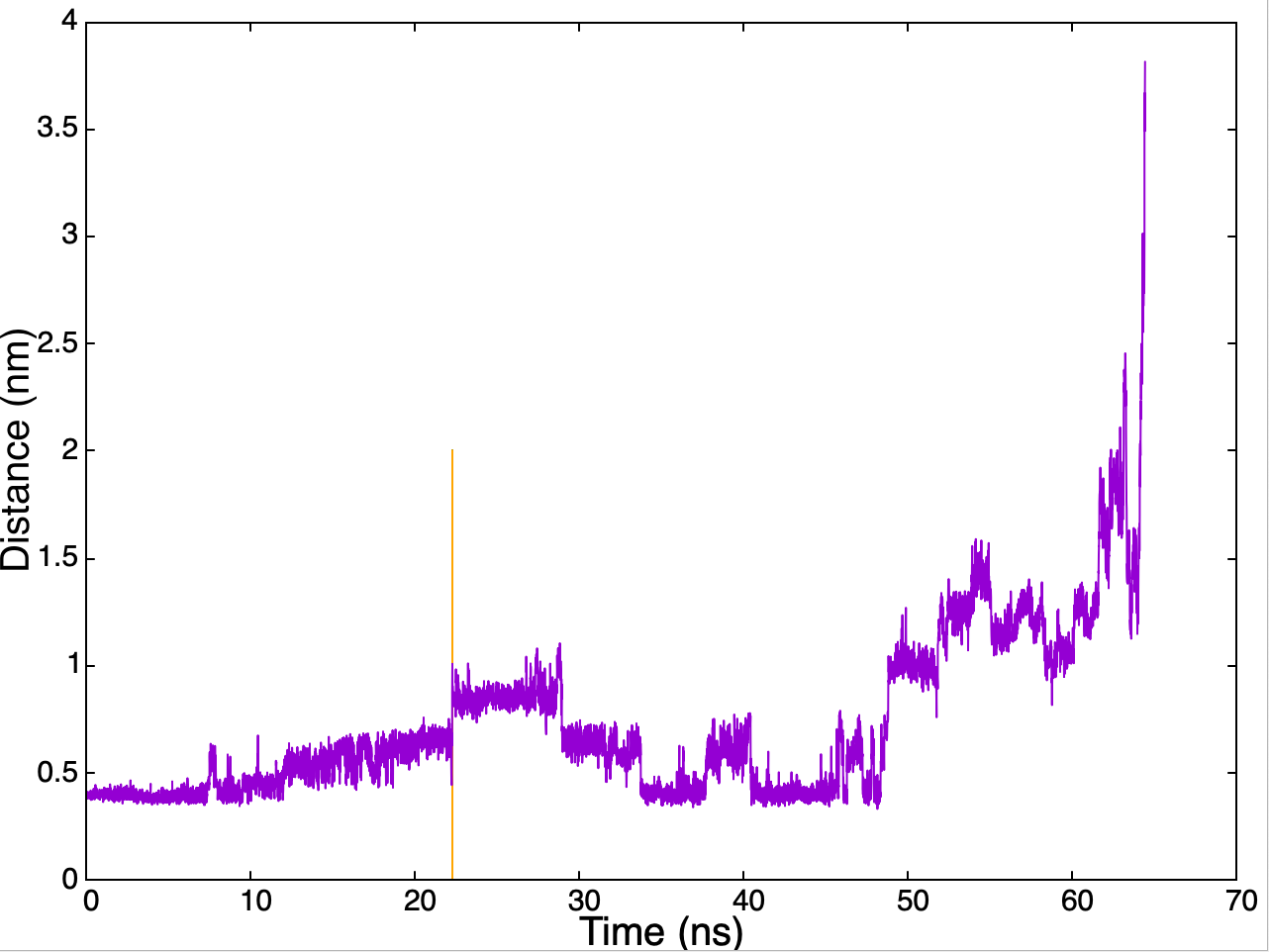
However, let's see an example to better understand what to do. In masterclass-22-1-infr we can see the sampling of the distance in one of the replica that was run for the benzamidine-trypsin system starting from the absolute minimum.
width 60%
Although the simulation lasted around 65 ns, our point of interest lies at around 22 ns (orange line), when we have a clear change in the sampling of the distance. Here, the absolute minimum was left thanks to the metadynamics bias added. We can measure the added bias up to that point by looking at the HILLS file. This information is important because, albeit low, the infrequent Metadynamics provides an acceleration booster to the simulation that must be estimated in order to extract the unbiased time for the transition.
The acceleration factor can be calculated using the following formula:
\[ \alpha = <e^{\beta V(s,t)}>, \]
where s is the collective variable of choice, \( \beta \) is the inverse of the Boltzmann constant multiplied the temperature in Kelvin, and V(s,t) is the bias felt at time t of transition [129]. Rescaling the transition time by this term will yield the real transition time that one would expect from an unbiased simulation. But how to obtain the characteristic transition time of the system starting from corrected transition times?
One practical way is to construct an empirical cumulative distribution function with the various corrected time values found in the independent replicas of infrequent Metadynamics. This is done by plotting on the x axis the time and on the y axis the percentage of simulations that evolved from our starting state to another. This scatter plot must then be fitted by a theoretical cumulative distribution function, which has the following equation:
\[ TCDF = 1 - exp(-t/\tau), \]
where t is our transition time and \( \tau \) is the characteristic transition time for the system of interest. The reliability of the fitting can be checked through the Kolmogorov-Smirnoff test.
The value thus obtained corresponds to the time requested on average for the system to move from our minimum to another well-defined state (state P) [129].
The same exercise can be done waiting for the ligand to leave the binding site, in which case we would be measuring the time requested for unbinding. The rate constant between the bound and unbound states can be approximated by dividing the number of transitions between the two by the total time the system spent in the bound state (calculated using the metadynamics simulation time and the acceleration factor as reported above).
This concludes the masterclass, thank you for your participation.
 1.8.17