 |
|
|
| |
|
|
This Masterclass explains how mechanical forces can be modeled using PLUMED, and the application of the FISST module for applying multiple forces simultaneously.
The objectives of this Masterclass are:
We assume that the person that will follow this tutorial is familiar with the Linux terminal, Gromacs and basic functionality of PLUMED.
Familiarity with python and matplotlib is recommended for FISST reweighting and plotting
We will use GROMACS, LAMMPS, PLUMED, and PLUMED's pesmd function to perform the calculations. Conda packages with the software required for this class have been prepared and you can install them following the instructions in this link.
If you are compiling PLUMED on your own, you will need to install the FISST module manually by adding '–enable-modules=fisst' to your './configure' command when building PLUMED.
The data needed to run the exercises of this Masterclass can be found on GitHub. You can clone this repository locally on your machine using the following command:
git clone https://github.com/hockyg/masterclass-22-15
A force along some direction here is defined as the negative gradient of the potential energy along that direction.
A constant force \(F\) on a scalar collective variable \(Q(\vec{X})\) therefore is a simple addition to the system's energy function.
\[ U(\vec{X},F) = U(\vec{X}) - F Q(\vec{X}) \]
Notice that, because of the negative sign, a postive value of \(F\) results in a lower energy for large values of \(Q\), meaning \(F\gt0\) corresponds to a "pulling" force.
A mechanical force would often in reality would correspond to pulling apart two atoms, and so \(Q\) would often be a simple distance coordinate.
Note however, that other quantities could be used, such as an area which would mean \(F\) corresponds to a pressure.
Dimensional analysis implies that the units of \(F\) must be [Energy]/[Q].
The effect of constant force can be assessed using any enhanced sampling method.
The work done by the bias in this case is very simple
\[ W = \int_a^b F \cdot d Q = F ( Q_b - Q_a ) \]
Constant forces can be applied in PLUMED with the SLOPE keyword of the RESTRAINT bias.
Steered molecular dynamics (SMD) is one way of pulling on a molecular coordinate, and has a connection to experiments done where a molecule is attached via a "spring" to an object such as an optical tweezer or AFM tip. To represent this in simulation, instead of applying a constant force, we impose a Harmonic restraint on \(Q\) with a center that moves:
\[ U(\vec{X},F) = U(\vec{X}) + \frac{1}{2} k (Q-Q_0(t))^2 \]
Typically \(Q_0(t)\) would move linearly, with \( Q_0(t) = Q_0(0)-\lambda t \) although that is not a requirement.
At any given time, the force along \(Q\) from the moving bias is given as:
\[ F(t) = -\frac{\partial U}{\partial Q} = -k(Q-Q_0(t)) \]
This force is positive (pulling) when \(Q_0(t)\) is bigger than \(Q\), and it can get very large if the spring moves quickly to larger values.
SMD is implemented in PLUMED using the MOVINGRESTRAINT bias, and the work is computed automatically.
\[ W = \int_a^B F dQ \approx \sum_{i=1}^{N_{steps}} \bar{F}_i (Q_0(t_i)-Q_0(t_{i-1})) = \lambda dt \sum_{i=1}^{N_{steps}} \bar{F}_i, \]
\[ \bar{F_i}=\frac{1}{2}( F_{i}+F_{i-1} ) = -\frac{k}{2}( Q(t_i)-Q_0(t_i) -Q(t_{i-1})+Q_0(t_{i-1})) = -\frac{k}{2} (\Delta Q_i - \lambda d t) \]
Infinite Switch Simulated Tempering in Force (FISST) is a method implemented in Ref. [64]
This method takes advantage of the limit of changing a force from \(F_{min}\) to \(F_{max}\) and back infinitely quickly.
In this limit, the system feels an average force \(\bar{F}(Q)\) that depends on the current value of the pulling coordinate.
\[ U(\vec{X},F) = U(\vec{X}) - \bar{F}(Q) Q(\vec{X}) \]
In practice, this \(\bar{F}(Q)\) is computed using weights \(w(F)\) for each force in the force range that are learned on the fly, and separate "observable weights" \(W_F(Q_i)\) are used to compute the average of any quantity \(A\) at a given force.
\[ \langle A \rangle_F = \frac{1}{N} \sum_{i=1}^{N_{steps}} A(X(t_i)) W_F(Q_i) \]
where the observable weights are computed in a way that
\[ W_F(Q_i)\propto \left(\int_{F_{min}}^{F_{max}} dF' w(F') e^{\beta (F'-F) Q_i} \right)^{-1} \]
The module writes out both the force weights and the observable weights to files.
The exercises are presented below.
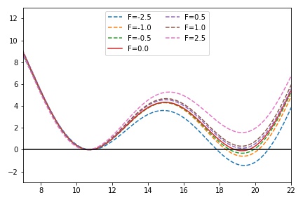
Use the RESTRAINT function to add a constant force of different magnitudes (e.g. -5 to 5 in these units) and look at how the force changes the resulting free energy surface.
UNITS ENERGYthe units of energy. =kcal/mol d1: DISTANCE ATOMSthe pair of atom that we are calculating the distance between. =1,2 ff: MATHEVAL ARGthe input for this action is the scalar output from one or more other actions. =d1 PERIODICcompulsory keyword if the output of your function is periodic then you should specify the periodicity of the function. =NO FUNCcompulsory keyword the function you wish to evaluate =0.2*(((x-10)^2)*((x-20)^2)) bb: BIASVALUE ARGthe input for this action is the scalar output from one or more other actions. =ff metad: METAD ARGthe input for this action is the scalar output from one or more other actions. =d1 PACEcompulsory keyword the frequency for hill addition =500 HEIGHTthe heights of the Gaussian hills. =0.1 SIGMAcompulsory keyword the widths of the Gaussian hills =2.5 FILEcompulsory keyword ( default=HILLS ) a file in which the list of added hills is stored =__FILL__ BIASFACTORuse well tempered metadynamics and use this bias factor. =10 TEMPthe system temperature - this is only needed if you are doing well-tempered metadynamics =300.0 GRID_WFILEthe file on which to write the grid =__FILL__ GRID_MINthe lower bounds for the grid =0 GRID_MAXthe upper bounds for the grid =30 GRID_BINthe number of bins for the grid =251 GRID_WSTRIDEwrite the grid to a file every N steps =10000 RESTRAINT __FILL__ PRINT ARGthe input for this action is the scalar output from one or more other actions. =* FILEthe name of the file on which to output these quantities =__FILL__ STRIDEcompulsory keyword ( default=1 ) the frequency with which the quantities of interest should be output =100
Then run the simulation using the command:
plumed pesmd < doublewell_prod.pesmd.input
Plot the free energy surface from the GRID or after using sum_hills to compute the surface, and zero the potential at the left minimum. What do you notice about the other minimum and barrier?
The following implements a "V-shaped" potential which has 2 minima at small y values and 1 minima at large y value.
Try plotting the potential to see.
d1: DISTANCE ATOMSthe pair of atom that we are calculating the distance between. =1,2 COMPONENTS( default=off ) calculate the x, y and z components of the distance separately and store them as label.x, ff: MATHEVAL ARGthe input for this action is the scalar output from one or more other actions. =d1.x,d1.y PERIODICcompulsory keyword if the output of your function is periodic then you should specify the periodicity of the function. =NO FUNCcompulsory keyword the function you wish to evaluate =-8*log((exp(-(y-exp(-x))^2/2)+exp(-(y+exp(-x))^2/2))*exp(-x^2/2)) bb: BIASVALUE ARGthe input for this action is the scalar output from one or more other actions. =ff PRINT ARGthe input for this action is the scalar output from one or more other actions. =* FILEthe name of the file on which to output these quantities =__FILL__ STRIDEcompulsory keyword ( default=1 ) the frequency with which the quantities of interest should be output =100
First run a simulation using the command, and make a 2d histogram of x and y to show that it is trapped on one side.
plumed pesmd < doublewell_prod.pesmd.input
If you have time, use RESTRAINT to add a constant force in the Y direction that favors the higher vertical state.
Now add FISST in order to sample forces all at once:
f: FISST MIN_FORCEcompulsory keyword Minimum force (per CV) to use for sampling. =-15 MAX_FORCEcompulsory keyword Maximum force (per CV) to use for sampling. =15.0 PERIODcompulsory keyword Steps corresponding to the learning rate =200 NINTERPOLATEcompulsory keyword Number of grid points on which to do interpolation. =41 ARGthe input for this action is the scalar output from one or more other actions. =d1.x KBTThe system temperature in units of KB*T. =1.0 OUT_RESTARTOutput file for all information needed to continue FISST simulation.If =__FILL__ OUT_OBSERVABLEOutput file putting weights needed to compute observables at different force values.If =__FILL__ OBSERVABLE_FREQHow often to write out observable weights (default=period). =100 CENTERcompulsory keyword ( default=0 ) The CV value at which the applied bias energy will be zero =0
We used forces -15 to 15 in the paper, but feel free to experiment with your own force range. Inspect the observable file and restart file to see what is in there.
Now generate a histogram at each force using the following command, which will render it as an animated gif if you have the proper libraries installed.
python reweight_vshape.py observable_file cv_file
In this section, we will study a toy model of a a helix using a bead spring model in lammps. This model has lowest energy when it is in a left or right handed helix, but it is not chiral, so they must have the same free energy.
First, run the system without any pulling, if you fisualize the trajectory, you will see that it is stuck in one configuration (epsilon sets the strength of the bonds, it can be studied at lower or higher stabilities by changing eps).
lmp -log helix_sf_example.log \
           -var plumed_file helix_sf_f-4.5_eps7.5_10000000.plumed.dat  \
           -var outprefix helix_sf_pull0 \
           -var steps 10000000  \
           -var eps 7.5 \
           -in run_helix_plumed.lmp
Now, run the system using FISST, suitibly modifying the plumed file to impose a force from -2 to 8 (as studied in the paper)
lmp -log helix_sf_example.log \
           -var plumed_file helix_fisst_fmin-2.0_fmax8.0_eps7.5_50000000.plumed.dat  \
           -var outprefix helix_fisst_fmin-2.0_fmax8.0_eps7.5_50000000 \
           -var steps 50000000  \
           -var eps 7.5 \
           -in run_helix_plumed.lmp
The included script 'compute_handedness.py' has an ad-hoc handedness calculation which is computed using RMSD to a left and right handed helix. The end-end distance is already computed in the colvars file.
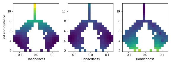
Use the handedness calculation in this script to create a 2d FES from the unbiased simulation, and from the unweighted FISST data.
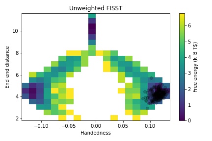
Note that both sides are equally explored in this relatively long simulation. Then compute plots reweighted to small/negative forces and large forces, and notice how the result mirrors that from the V-shaped potential.
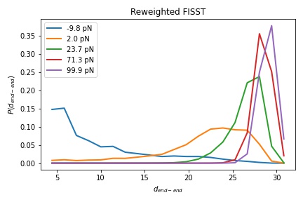
We will now study the effect of force on a model peptide, alanine 10 in water. You can set this up to run yourself, but the colvar files are also included for a 200ns simulation of alanine 10 run with FISST from forces -10 to 10 pN and from -10 to 100 pN.
Note, now we are using real units, a conversion factor is needed: 69.4786 pN = 1 kcal/mol/Angstrom
To run yourself, modify ala10_fisst.plumed.dat
gmx_mpi -s ala10.tpr -plumed ala10_fisst.plumed.dat -nsteps 100000000 --deffnm OUTPUT_PREFIX
Then analyze your files, or my files ala10_pull_fRange_fmin-10_fmax100.* to compute the end-end distance of Alanine 10 at different forces. Do your results from different FISST ranges agree?
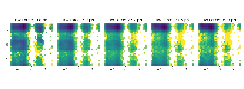
Finally, use the observable weights to compute the Ramachandran plot (averaged over residues) at different forces (mine is from analyzing the gromacs structural output, but you may want to put the phi-psi calculation in the plumed file as in previous tutorials!)
 1.8.17