 |
|
|
| |
|
|
Much of this exercise was originally created by Alberto Pérez de Alba Ortíz for the Cecam School "Understanding Molecular Simulation", held annually in Amsterdam.
The aim of this Masterclass is to demonstrate the advantages of path collective variables for describing and simulating activated molecular processes, and to provide hands-on experience with setting up, running, and analyzing biased path-CV simulations, such as path-metadynamics.
Once this Masterclass is completed, users will be able to:
We assume that you are familiar with PLUMED. However, the 2021 PLUMED Masterclass is a great place to start if you are not.
The data needed to complete the exercises of this Masterclass can be found on GitHub. You can clone this repository locally on your machine using the following command:
git clone https://github.com/Ensing-Laboratory/masterclass-22-09
We will use Plumed version 2.3.0 for this exercise together with personal versions of the PathCV and PESMD features. With the above git clone command, you have already downloaded them, and with the following commands we compile this version of plumed:
cd masterclass-22-09/plumed
chmod +x install
./install
This takes about 5-10 minutes on a modern laptop or desktop computer. After that, the plumed executable is installed in the folder masterclass-22-09/plumed/bin.
Information on these versions of the PathCV option and the PESMD option may be slightly different from that in the latest online plumed manual. Instead, open your local version in a browser, which you can find in the following locations on your computer:
masterclass-22-09/plumed/plumed-2.3.0/user-doc/html/index.htmlmasterclass-22-09/plumed/plumed-2.3.0/user-doc/html/pesmd.htmlmasterclass-22-09/plumed/plumed-2.3.0/user-doc/html/_p_a_t_h_c_v.htmlThe exercises are found in the folder masterclass-22-09/exercises.
In this exercise, we will perform metadynamics [1] and path-metadynamics (PMD) [2-4] simulations of a system that can undergo a transition between two free energy minima. These two stable states are separated by a transition state barrier, so that the transition process is a rare event for `‘normal’' (i.e. unbiased) molecular dynamics simulations.
PMD is able to simultaneously and efficiently converge the transition path (which can be either an average transition path or a minimum free energy path (MFEP)) and the free energy profile of the process along this path. This is achieved by performing metadynamics on an adaptive path connecting the two known stable states.
In order to understand the principles and advantages of PMD, we will first perform standard metadynamics and get familiar with its parameters and functionalities. Subsequently, we will add the features corresponding to the adaptive path. To ease computation and visualization, we will employ a simple model system.
This exercise makes use of PLUMED's [5] own internal engine: plumed pesmd, i.e. without being coupled to an MD engine that runs an actual molecular system. The advantages are that the simulations will be very fast, and you do not need to know anything about the MD engine of our choice, which might be different from the one that you are used to.
Still, the enhanced sampling techniques that you will use in this exercise, and the plumed input files that we will write for that, can also be used (with very little changes) with plumed patched to any MD software, which means that you can potentially use it for your own research!
In order to overcome the timescale limitations of MD and be able to observe relevant molecular transitions, the community has developed a plethora of enhanced sampling methods. Among them, we can identify the so-called biasing methods, which work by exerting an external potential (or force) on a few key descriptive degrees of freedom of the transition, commonly called collective variables (CVs).
The choice and design of CVs is a task of great importance. In the following, we will assume that the CVs are known. We will consider a molecular system whose free energy surface (FES) is fully described by a set of \(N\) CVs, \(\{z_i(\mathbf{q}\,)\}\) with \(i=1... N\), which are all functions of the system's particle positions \(\mathbf{q}(t)\). We will also assume that these particle positions \(\mathbf{q}(t)\) evolve in time with a canonical equilibrium distribution at temperature \(T\) under a potential \(V(\mathbf{q})\).
We are interested in exploring the space spanned by the CVs, \(\{z_i\}\), and in quantifying the free energy. In order to do so, in metadynamics we exert a history-dependent repulsive potential by summing Gaussian kernels over time:
\[ V_\text{bias}(\mathbf{z},t) = \sum_{\kappa\tau<t} H(\kappa\tau) \exp \biggr( - \sum^{N}_{i=1} \frac{(z_i - z_i(q(\kappa\tau)))^2}{2 W_i^2} \biggr), \]
with Gaussian height \(H\), widths along each CV \(W_i\), and depositing frequency \(\tau\). This bias drives the system away from already visited configurations and into new regions of CV-space. More importantly, in the long-time limit, the bias potential converges to the minus free energy as function of the CVs: \(V_\text{bias}(\mathbf{z},t \rightarrow \infty) = - F(\mathbf{z})\).
As a well-established sampling technique, metadynamics also has several extensions to accelerate convergence and improve computational performance, such as the multiple-walker and well-tempered versions [6,7].
Metadynamics can handle a few CVs simultaneously in a trivial manner, which spares us from having to find a single perfect CV. Instead, an appropriate set of CVs allows us to converge an insightful multidimensional free energy landscape, in which (meta)stable states and connecting MFEPs can be identified. In practice however, especially when investigating complex transitions, the number of CVs is limited to \(N\approx3\), because of the exponential growth of computational cost with CV dimensionality.
In order to tackle complex transitions that require many CVs, path-based methods were developed. In these schemes, a path-CV is introduced. That is, a parametrized curve that connects two FES basins — the known stable states \(A\) and \(B\) — in the space spanned by the CVs: \(\mathbf{s}(\sigma): \mathbb{R} \rightarrow \mathbb{R}^N\), where the parameter \(\sigma(\mathbf{z}\,) | _{s} : \mathbb{R}^N \rightarrow [0,1]\) yields the progress along the path from \(A\) to \(B\), such that \(\mathbf{s}(0) \in A\) and \(\mathbf{s}(1) \in B\).
This progress parameter emulates the reaction coordinate and can in principle be connected to the committor value. Since the transition path curve is not known a priori, the path-CV must be adaptive. If we assume that, in the vicinity of the path, the iso-commitor planes \(S_\sigma\) are perpendicular to \(\mathbf{s}(\sigma)\), and that the configurational probability is a good indicator of the transition flux density, then we can converge the average transition path by iteratively adapting a guess path to the cumulative average density: \(\mathbf{s}_g(\sigma_g) = \langle\mathbf{z}\,\rangle _{\sigma_g}\) [3].
The key advantage of PMD is that the metadynamics biasing can be performed on the 1D progress parameter along the adaptive path-CV, instead of the \(N\)-dimensional CV-space. PMD is able to converge a path, and the free energy along it, with a sublinear rise in computational cost with respect to the growth in CV dimensionality (instead of the exponential relation when not using a path-CV)[4].
Numerically, the adaptive path-CV is implemented as a set of \(M\) ordered nodes (coordinates in CV-space) \(\mathbf{s}_g (\sigma_g,t) \rightarrow {\mathbf{s}^{\,t_i}_j}\) with \(j=1,...,M\), where \(t_i\) is the discrete time of path updates. The projection of any point \(\mathbf{z}\) onto the path is done considering the closest two nodes, and \(\sigma\) is obtained by interpolation. This approach requires equidistant nodes, which are imposed by a reparametrization step after each path update. The update step for the path nodes is done by:
\[ \mathbf{s}_j^{\,t_{i+1}} = \mathbf{s}_j^{\,t_{i}} + \frac{ \sum_k^{} w_{k} \cdot ( \mathbf{z}_k - \mathbf{s}^{\,t_{i}} ( \sigma (\mathbf{z}_k) ) )} { \sum_k^{} \xi^{t_i - k} w_{j,k} }, \text{ with } \\ w_{k} = \max \biggr[ 0, \biggr( 1 - \frac{|| \mathbf{s}^{\,t_i}_j - \mathbf{s}^{\,t_i} (\sigma ( \mathbf{z}_k)) ||}{|| \mathbf{s}^{\,t_i}_j - \mathbf{s}^{\,t_i}_{j+1} ||} \biggr) \biggr], \]
where \(k\) is the current MD step and \(w\) is the weight of the adjustment, which is non-zero only for the two nodes closest to the average CV density. We also introduce the fade factor \(\xi =\exp( -\ln(2) / \tau_{1/2})\), with \(\tau_{1/2}\) as a half-life: the number of MD steps after which the distances measured from the path weight only 50% of its original value. A short half-life increases path flexibility by allowing it to rapidly `‘forget’' a bad initial guess, while a long half-life restricts the path fluctuations and leads eventually to optimal convergence. The first and last nodes, located at the stable states \(A\) and \(B\) respectively, remain fixed. Extra trailing nodes can be placed at both ends of the path to better capture the free energy valleys. Wall potentials can be used to keep the sampling near the relevant [0,1] \(\sigma\)-interval.
Additionally, a harmonic restraint set on \(|| \mathbf{z}_k - \mathbf{s}^{\,t_{i}} ( \sigma (\mathbf{z}_k) ) ||\) can help in converging to a specific transition path in scenarios with multiple or ill-defined transition channels. We refer to this restraint as a `‘tube’' potential. In the limit of an infinitesimally narrow tube potential, the path update step follows the local free energy gradient and PMD converges to the MFEP instead of the average transition path. This control over the behavior of the algorithm is an advantageous feature, as switching from a density-driven to a gradient-driven path optimization leads either to the average transition path or the MFEP.
Metadynamics, the method of choice to sample the path-CV, drives the system back and forth along the path, providing sufficient sampling of the CV density to localize the transition path. At the same time, metadynamics continuously self-corrects the free energy by overwriting the previously deposited Gaussians with new ones. This leads to a converged free energy along the localized path: \(V_\text{bias}(\sigma,t \rightarrow \infty) = -F(\sigma)\). Most of the algorithmic extensions developed for metadynamics (well-tempered, transition-tempered, multiple walkers, etc.) can be straightforwardly combined with the adaptive path-CV. Moreover, other biasing techniques (umbrella sampling, constrained MD, steered MD, etc.) can also be used to sample along the path, or even in the direction perpendicular to it.
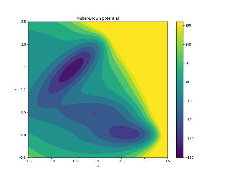
In this exercise, we will sample the well-known Müller-Brown (MB) potential energy surface (PES). You can find more about it in Ref. [8]. We add harmonic walls to limit the sampling within the interesting region of the PES.
To install PLUMED, if you have not already done this above, go to the folder plumed in the folder for this exercise. In the script install, change the prefix to the installation folder of your choice, and then run the script. If you have issues with the installation you can check: https://plumed.github.io/doc-v2.3/user-doc/html/_installation.html
To visualize the results of this exercise, plotting script examples are provided for the gnuplot plotting software (see the script files names starting with plot_ or anim_). Make sure to change the corresponding variables according to your choices of the metadynamics and path-CV parameters. Of course, feel free to use other plotting tools, for example pythons matplotlib.
To run the PLUMED pesmd on the MB PES, use the command plumed pesmd < path/to/input. The input file is located in the Exercise folder. Review the PLUMED pesmd documentation: https://plumed.github.io/doc-v2.4/user-doc/html/pesmd.html. To perform metadynamics, you can review the keywords on: https://plumed.github.io/doc-v2.3/user-doc/html/_m_e_t_a_d.html. To use the adaptive path-CV, you can review the keywords in the header of the file PathCV.cpp in the folder plumed in the folder for this exercise. To see the html documentation on the path-CV in a browser, open <PMD_exercise/plumed/plumed-2.3.0/user-doc/html/_p_a_t_h_c_v.html> in a browser. To construct a FES from the metadynamics hills, use the plumed sum\_hills functionality. Consult its features on: https://plumed.github.io/doc-v2.3/user-doc/html/sum_hills.html. We recommend to use --stride 1 and --mintozero.
The first exercise is found in the folder: masterclass-22-09/exercises/0_md.
This first exercise is meant to get acquainted with running the plumed pesmd engine, understanding the input files, and plotting the MD trajectory in the MB potential from the colvar file using gnuplot (or other plotting software). To use the ./run.me script to start the simulation, first make the script executable using:
chmod +x ./run.me
Use PLUMED pesmd to run regular MD on the MB PES.
What do you observe?
How would you change the behaviour of the system without using an enhanced sampling method (just modifying the MD run parameters)?
This exercise is found in the folder: masterclass-22-09/exercises/1_metadynamics.
Before you can run the metadynamics simulation, the plumed.dat should be completed:
UNITS LENGTHthe units of lengths. =nm TIMEthe units of time. =fs cv: DISTANCE ATOMSthe pair of atom that we are calculating the distance between. =1,2 COMPONENTS( default=off ) calculate the x, y and z components of the distance separately and store them as label.x, lwall: LOWER_WALLS ARGthe input for this action is the scalar output from one or more other actions. =cv.x,cv.y ATcompulsory keyword the positions of the wall. =-1.5,-0.5 KAPPAcompulsory keyword the force constant for the wall. =1000.0,1000.0 uwall: UPPER_WALLS ARGthe input for this action is the scalar output from one or more other actions. =cv.x,cv.y ATcompulsory keyword the positions of the wall. =1.5,2.5 KAPPAcompulsory keyword the force constant for the wall. =1000.0,1000.0 metad: ### ADD could not find this keyword YOUR could not find this keyword METADYNAMICS could not find this keyword INSTRUCTIONS could not find this keyword HERE could not find this keyword PRINT ARGthe input for this action is the scalar output from one or more other actions. =cv.x,cv.y,metad.bias STRIDEcompulsory keyword ( default=1 ) the frequency with which the quantities of interest should be output =100 FILEthe name of the file on which to output these quantities =colvar.out USE PLUMED could not find this keyword pesmd could not find this keyword to could not find this keyword run could not find this keyword metadynamics could not find this keyword on could not find this keyword the could not find this keyword MB could not find this keyword PES. could not find this keyword
Here are some hints for defining the METAD rule:
DISTANCE components cv.x and cv.y, which are actually the coordinates of a "2D particle" (with respect to the origin) undergoing a Langevin dynamics on the MB PES. Use these components as the ARG arguments in the METAD rule.SIGMA) are ca. 0.1.FILE, that can afterward be read using plumed sum_hills to generate and plot the free energy landscape.Try to obtain a good FES reflecting the two minima.
Vary the width of the Gaussians for each CV in a systematic manner, what effect do you observe?
Vary the height and deposition frequency of the Gaussians, what trends do you observe?
How many crossings and recrossings do you sample in a single run for each choice of parameters?
This exercise is found in the folder: masterclass-22-09/exercises/2_fixedpathmetadynamics.
Run metadynamics along a fixed path-CV on the MB PES. We recommend using 20 transition nodes, with 20 trailing nodes at each end (60 nodes in total). Use harmonic walls to keep the sampling within a relevant [-0.2,1.2] \(\sigma\)-range.
Now there's only one dimension for the Gaussian width, how do you interpret it?
Does the diffusion of the system along \(\sigma\) reflect anything particular? What could be the reason?
What happens if you add and strengthen a tube potential?
What is the final path and free energy that you obtain?
This exercise is found in the folder: masterclass-22-09/exercises/3_adaptivepathmetadynamics.
First, change the plumed.dat input file to make the path adaptive by changing PACE, STRIDE, and HALFLIFE.
Run metadynamics along an adaptive path-CV on the MB PES. For simplification, start with the same pace for the metadynamics Gaussians and the path update.
For simplification, you can keep only 20 transition nodes, and not use trailing nodes.
Use harmonic walls to keep the sampling within a relevant [-0.2,1.2] \(\sigma\)-range.
What do you expect if you vary the ratio between the metadynamics and the path update frequency?
Vary the tube potential strength and the half-life parameter, what trend do you observe?
A small value for the HALFLIFE (say 1000 MD steps), keeps the path flexible so that the path evolves efficiently away from a poor initial guess path. However, once it has reached the transition channel, it would be better to set it to a very large value, in order to converge to the average transition path. Run first a short PMD simulation using a flexible path and relatively large Gaussians, until the system has filled both basins and has recrossed back to the initial state. Then, restart the simulation, using smaller Gaussians and a large halflife. Use the INFILE directive (instead of GENPATH) to read the last updated path, which can be taken from the tail of the path.out file of the first run.
This exercise is found in the folder: masterclass-22-09/exercises/4_multiplewalkers.
In this final exercise, you will run the parallel "multiple walker" version of path-metadynamics.
Note that with more walkers building the metadynamics simulation, the total run time can be shorter, and possibly also the Gaussians can be smaller.
Try several configurations of walkers and try to answer the question if there is an optimal number of walkers.
[1] A. Laio and M. Parrinello, “Escaping free-energy minima,” Proc. Natl. Acad. Sci. USA, vol. 99, no. 20, pp. 12562–12566, 2002.
[2] D. Branduardi, F. Gervasio, and M. Parrinello, “From A to B in free energy space,” J. Chem. Phys, vol. 126, p. 054103, 2007.
[3] G. Díaz Leines and B. Ensing, “Path finding on high-dimensional free energy landscapes,” Phys. Rev. Lett., vol. 109, no. 2, p. 020601, 2012.
[4] A. Pérez de Alba Ortíz, A. Tiwari, R. C. Puthenkalathil, and B.Ensing, “Advances in enhanced sampling along adaptive paths of collective variables,” _ J. Chem. Phys._, vol. 149, no. 7, p. 072320, 2018.
[5] G. A. Tribello, M. Bonomi, D. Branduardi, C. Camilloni, and G. Bussi, “Plumed2:Newfeathers for an old bird,” Comp. Phys. Comm., vol. 185, no. 2, pp. 604–613, 2014.
[6] P. Raiteri, A. Laio, F. L. Gervasio, C. Micheletti, and M. Parrinello, “Efficient reconstruction of complex free energy landscapes by multiple walkers metadynamics,” J. Phys. Chem. B., vol. 110, no. 8, pp. 3533–3539, 2006.
[7] A. Barducci, G. Bussi, and M. Parrinello, “Well-tempered metadynamics: a smoothly converging and tunable free-energy method,” Phys. Rev. Lett., vol. 100, no. 2, p. 020603, 2008.
[8] K. Müller and L. D. Brown, “Location of saddle points and minimum energy paths by a constrained simplex optimization procedure,” Theor. Chim. Acta, vol. 53, no. 1, pp. 75–93, 1979.
 1.8.17