 |
|
|
In this section we want to introduce the concept of adaptive collective variables. These are special variables that are knowledge-based in that are built from a pre-existing notion of the mechanism of the transition under study
Here is the tarball with the files referenced in the following.
When you deal with a complex conformational transition that you want to analyze (or bias), very often you cannot just describe it with a single order parameter.
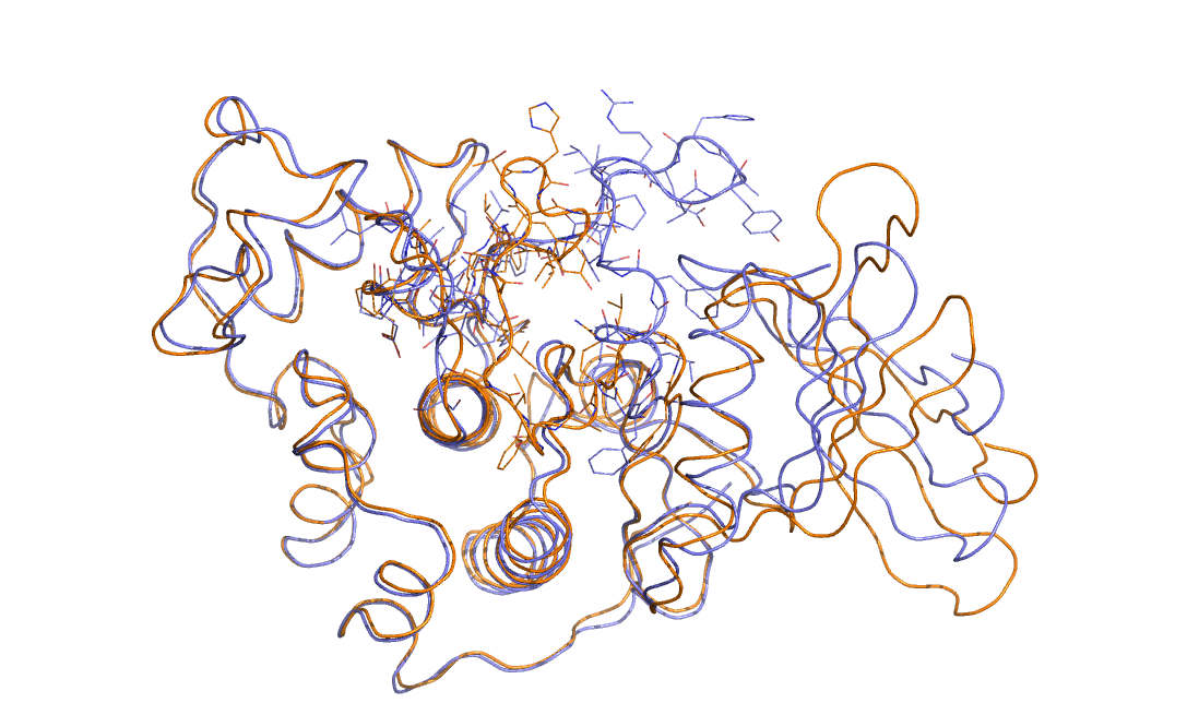
As an example in Figure belfast-2-cdk-fig I consider a large conformational transition like those involved in activating the kinase via open-close transition of the activation loop. In sticks you see the part involved in the large conformational change, the rest is either keeping the structure and just moving a bit or is a badly resolved region in the X-ray structure. This is a complex transition and it is hard to tell which is the order parameter that best describes the transition.
One could identify a distance that can distinguish open from close but
So basically in these cases you have to deal with an intrinsic multidimensional collective variable where you would need many dimensions. How would you visualize a 10 dimensional CV where you use many distances, coordinations and dihedrals (ouch, they're periodic too!) ?
Another typical case is the docking of a small molecule in a protein cleft or gorge, which is the mechanism of drug action. This involves specific conformational transition from both the small molecule and the protein as the small molecule approaches the protein cavity. This also might imply a specific desolvation pattern.
Other typical examples are chemical reactions. Nucleophiloic attacks typically happen with a role from the solvent (see some nice paper from Nobel-prize winner Arieh Warshel) and sizeable geometric distortions of the neighboring groups.
One possibility to describe many different thing that happen in a single reaction is to use a dimensional reduction technique and in plumed the simplest example that may show its usefulness can be considered that of the path collective variables.
In a nutshell, your reaction might be very complex and happening in many degree of freedom but intuitively is a sort of track along which the reaction proceeds. So what we need is a coordinate that, given a conformation, just tells which point along the "reactive track" is closest.
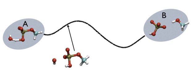
For example, in Fig. belfast-2-ab-fig, you see a typical chemical reaction (hydrolisys of methylphosphate) with the two end-points denoted by A and B. If you are given a third point, just by looking at it, you might find that this is more resemblant to the reactant than the product, so, hypothetically, if you would intuitively give a parameter that would be 1 for a configuration in the A state and 2 for a configuration in the B state, you probably would give it something like 1.3, right?
Path collective variables are the extension to this concept in the case you have many conformation that describe your path, and therefore, instead of an index that goes from 1 to 2 you have an index that goes from 1 to \(N\) , where \(N\) is the number of conformation that you use in input to describe your path.
From a mathematical point of view, that's rather simple. The progress along the path is calculated with the following equation:
\[ S(X)=\frac{\sum_{i=1}^{N} i\ \exp^{-\lambda \vert X-X_i \vert }}{ \sum_{i=1}^{N} \exp^{-\lambda \vert X-X_i \vert } } \]
where in belfast-2-s-eq the \( \vert X-X_i \vert \) represents a distance between one configuration \( X \) which is analyzed and another from the set that compose the path \( X_i \). The parameter \( \lambda \) is a positive value that is tuned in a way explaned later. here are a number of things to note to make you think that this is exactely what you want.
In order to provide a value which is continuous, the parameter \( \lambda \) should be correclty tuned. As a rule of thumb I use the following formula
\[ \lambda=\frac{2.3 (N-1) }{\sum_{i=1}^{N-1} \vert X_i-X_{i+1} \vert } \]
which imply that one should calculate the average distance between consecutive frames composing the path. Note also that this distance should be more or less similar between the frames. Generally I tolerate fluctuation of the order of 10/15 percent tops. If you have larger, then it is better to have a smaller value of \( \lambda \).
It is important to note that in principle one could even have a specific \( \lambda \) value associated to each frame of the path but this would provide some distortion in the diffucion coefficient which could potentially harm a straightforward interpretation of the free energy landscape.
So, at this point is better to understand what is meant with "distance" since a distance between two conformations can be calculated in very many ways. The way we refer here is by using mean square deviation after optimal alignment. This means that at each step in which the analisys is performed, a number N of optimal alignments is performed. Namely what is calculated is \( \vert X-X_i \vert = d(X,X_i)^2 \) where \( d(X,X_i) \) is the RMSD as defined in what you see here RMSD.
Using the MSD instead of RMSD is sometimes more convenient and more stable (you do not have a denominator that gies to zero in the derivatives when biasing.
Anyway this is a matter of choice. Potentially one could equally employ other metrics like a set of coordinations (this was done in the past), and then you would avoid the problem of rototranslations (well, which is not a problem since you have it already in plumed) but for some applications that might become appealing. So in path collective variables (and in all the dimensional reduction based collective variables) the problem is converted from the side of choosing the collective variable in choosing the right way to calculate distances, also called "metrics".
The discussion of this issue is well beyond the topic of this tutorial, so we can move forward in how to tell plumed to calculate the progress along the path whenever the MSD after optimal alignment is used as distance.
p1: PATHMSD REFERENCE=all.pdb LAMBDA=50.0
PRINT ARG=p1.sss,p1.zzz STRIDE=100 FILE=colvar FMT=%8.4f
Note that reference contains a set of PDB, appended one after the other, with a END field. Note that there is no need to place all the atoms of the system in the PDB reference file you provide. Just put the atoms that you think might be needed. You can leave out big domains, solvent and ions if you think that is not important for your use.
Additionally, note that the measure units of LAMBDA are in the units of the code. In gromacs they are in nm^2 while NAMD is Ang^2. PATHMSD produces two arguments that can be printed or used in other ActionWithArguments. One is the progress along the path of belfast-2-s-eq, the other is the distance from the closest point along the path, which is denoted with the zzz component. This is defined as
\[ Z(X)=-\frac{1}{\lambda}\log (\sum_{i=1}^{N} \ \exp^{-\lambda \vert X-X_i \vert }) \]
It is easy to understand that in case of perfect match of \( X=X_i \) this equation gives back the value of \( \vert X-X_i \vert \) provided that the lambda is adjusted correctly.
So, the two variables, put together can be visualized as
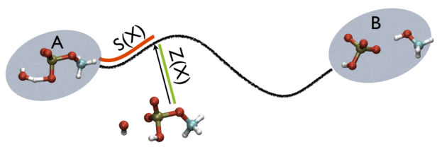
This variable is important because whenever your simulation is running close to the path (low Z values), then you know that you are reproducing reliably the path you provided in input but if by chance you find some other path that goes, say, from \( S=1, Z=0 \) to \( S=N, Z=0 \) via large Z values, then it might well be that you have just discovered a good alternative pathway. If your path indeed is going from \( S=1, Z=large \) to \( S=N, Z=large \) then it might well be that you do not have your reaction accomplished, since your reaction, by definition should go from the reactant which is located at \( S=1, Z=0 \) to the product, which is located at \( S=1, Z=N \) so you should pay attention. This case is exemplified in Fig. belfast-2-ab-sz-nowhere-fig
A truly important point is that if you get a trajectory from some form of accelerated dynamics (e.g. simply by heating) this cannot simply be converted into a path. Since it is likely that your trajectory is going stochastically back and forth (not in the case of SMD or US, discussed later), your trajectory might be not topologically suitable. To understand that, suppose you simply collect a reactive trajectory of 100 ps into the reference path you give to the PATHMSD and simply you assign the frame of 1 ps to index 1 (first frame occurring in the reference file provided to PATHMSD), the frame of 2 ps to index 2 and so on : it might be that you have two points which are really similar but one is associated to step, say 5 and the other is associated with frame 12. When you analyse the same trajectory, when you are sitting on any of those points then the calculation of S will be an average like \( S(X)=(5+12)/2=8.5 \) which is an average of the two indexes and is completely misleading sinec it let you think that you are moving between point 8 and 9, which is not the case. So this evidences that your reference frames should be "topologically consecutive". This means that frame 1 should be the closest to frame 2 and all the other frames should be farther apart. Similarly frame 2 should be equally close (in an RMSD sense) to 1 and 3 while all the others should be farther apart. Same for frame 3: this should be closest to frame 2 and 4 and farther apart from all the others and so on. This is equivalent to calculate an "RMSD matrix" which can be conveniently done in vmd (this is a good exercise for a number of reasons) with RMSD Trajectory tools, by choosing different reference system along the set of reference frames.
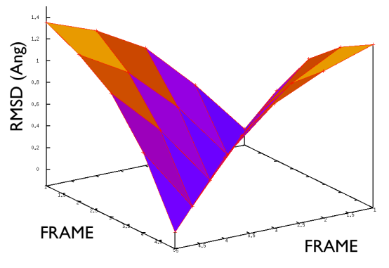
This is shown in Fig. belfast-2-good-matrix-fig where the matrix has a typical gullwing shape.
On the contrary, whenever you extract the frames from a pdb that you produced via free MD or some biased methods (SMD or Targeted MD for example) then your frame-to-frame distance is rather inhomogeneous and looks something like
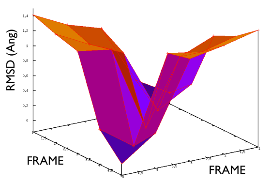
Aside from the general shape, which is important to keep the conformation-to-index relation (this, as we will see in the next part is crucial in the multidimensional scaling) the crucial thing is the distance between neighbors.
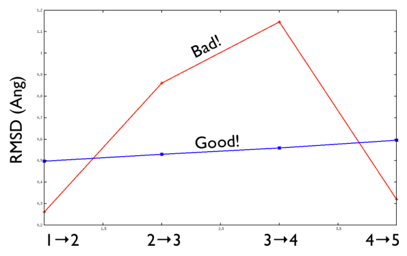
As a matter of fact, this is not much important in the analysis but is truly crucial in the bias. When biasing a simulation, you generally want to introduce a force that push your system somewhere. In particular, when you add a bias which is based on a path collective variable, most likely you want that your system goes back and forth along your path. The bias is generally applied by an additional term in the hamiltonian, this can be a spring term for Umbrella Sampling, a Gaussian function for Metadynamics or whatever term which is a function of the collective variable \( s \). Therefore the Hamiltonian \( H (X) \) where \( X \) is the point of in the configurational phase space where your system is takes the following form
\[ H'(X)=H(X)+U(S(X)) \]
where \( U(S(X)) \) is the force term which depends on the collective variable that ultimately is a function of the \( X \). Now, when you use biased dynamics you need to evolve according the forces that this term produces (this only holds for MD, while not in MC) and therefore you need
\[ F_i=-\frac{d H'(X) }{d x_i} = -\frac{d H'(X) }{d x_i} -\frac{\partial U(S(X)) }{ \partial S}\frac{\partial S(X)}{\partial x_i} \]
This underlines the fact that, whenever \( \frac{\partial S(X)}{\partial x_i} \) is zero, then you have no force on the system. Now the derivative of the progress along the path is
\[ \frac{\partial S(X) }{\partial x_i} =\frac{\sum_{i=1}^{N} -\lambda\ i\ \frac{\partial \vert X-X_i \vert}{ \partial x_i} \exp^{-\lambda \vert X-X_i \vert }}{ \sum_{i=1}^{N} \exp^{-\lambda \vert X-X_i \vert } } - \frac{ (\sum_{i=1}^{N} i\ \exp^{-\lambda \vert X-X_i \vert } ) (\sum_{j=1}^{N} -\lambda \frac{\partial \vert X-X_j \vert}{ \partial x_i} \exp^{-\lambda \vert X-X_j \vert } ) }{ ( \sum_{i=1}^{N} \exp^{-\lambda \vert X-X_i \vert } )^2} = \frac{\sum_{i=1}^{N} -\lambda\ i\ \frac{\partial \vert X-X_i \vert}{ \partial x_i} \exp^{-\lambda \vert X-X_i \vert }}{ \sum_{i=1}^{N} \exp^{-\lambda \vert X-X_i \vert } } -s(X) \frac{ (\sum_{j=1}^{N} -\lambda \frac{\partial \vert X-X_j \vert}{ \partial x_i} \exp^{-\lambda \vert X-X_j \vert } ) } {\sum_{i=1}^{N} \exp^{-\lambda \vert X-X_i \vert } } \]
\[ \frac{\partial S(X) }{\partial x_i} = \lambda \frac{\sum_{i=1}^{N} \frac{\partial \vert X-X_i \vert}{ \partial x_i} \exp^{-\lambda \vert X-X_i \vert } [ s(X) - i ] } { \sum_{i=1}^{N} \exp^{-\lambda \vert X-X_i \vert } } \]
It is interesting to note that whenever the \( \lambda \) is too small the force will vanish. Additionally, when \( \lambda \) is too large, then it one single exponential term will dominate over the other on a large part of phase space while the other will vanish. This means that the \( S(X) \) will assume almost discrete values that produce zero force. Funny, isn't it?
A very common question that comes is the following: "I have my reaction or a model of it. how many frames do I need to properly define a path collective variable?" This is a very important point that requires a bit of thinking. It all depends on the limiting scale in your reaction. For example, if in your process you have a torsion, as the smallest event that you want to capture with path collective variable, then it is important that you mimick that torsion in the path and that this does not contain simply the initial and final point but also some intermediate. Similarly, if you have a concerted bond breaking, it might be that all takes place in the range of an Angstrom or so. In this case you should have intermediate frames that cover the sub-Angstrom scale. If you have both in the same path, then the smallest dominates and you have to mimick also the torsion with sub-Angstrom accuracy.
If it happens that you have a very complex and detailed path to use, say that it contains 100 frames with 200 atoms each, then the calculation of a 100 alignment is required every time you need the CV. This can be quite expensive but you can use a trick. If your trajectory is continuous and you are sure that your trajectory does not show jumps where your system suddedly move from the reactant to the product, then you can use a so-called neighbor list. The plumed input shown before then becomes
p1: PATHMSD REFERENCE=all.pdb LAMBDA=50.0 NEIGH_STRIDE=100 NEIGH_SIZE=10
PRINT ARG=p1.sss,p1.zzz STRIDE=100 FILE=colvar FMT=%8.4f
and in this case only the closest 10 frames from the path will be used for the CV. Then the list of the frames to use is updated every 100 steps. If you are using a biased dynamics this may introduce sudden change in the derivatives, therefore it is better to check the stability of the setup before running production-quality calculations.
Here and probably in other parts of the tutorial a simple molecule is used as a test case. This is alanine dipeptide in vacuum. This rather simple molecule is useful to make many benchmark that are around for data analysis and free energy methods. It is a rather nice example since it presents two states separated by a high (free) energy barrier.
In Fig. belfast-2-ala-fig its structure is shown.
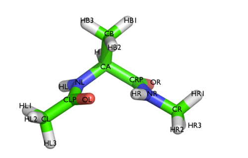
The two main metastable states are called \( C_7eq \) and \( C_7ax \).
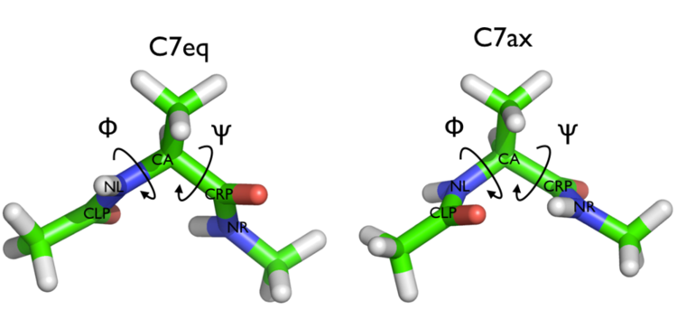
Here metastable states are intended as states which have a relatively low free energy compared to adjacent conformation. At this stage it is not really useful to know what is the free energy, just think in term of internal energy. This is almost the same for such a small system whith so few degrees of freedom.
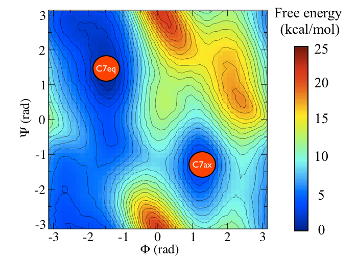
It is conventional use to show the two states in terms of Ramachandran dihedral angles, which are denoted with \( \Phi \) and \( \Psi \) in Fig. belfast-2-transition-fig .
Now as a simple example, I want to show you that plotting some free dynamics trajectories shoot from the saddle point, you get a different plot in the path collective variables if you use the right path or if you use the wrong path.
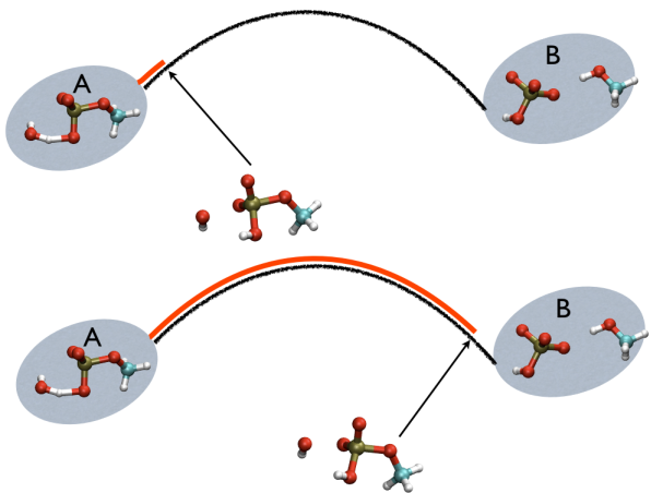
In Fig. belfast-2-good-bad-path-fig I show you two example of possible path that join the \( C_7eq \) and \( C_7ax \) metastable states in alanine dipeptide. You might clearly expect that real (rare) trajectories that move from one basin to the other would rather move along the black line than on the red line.
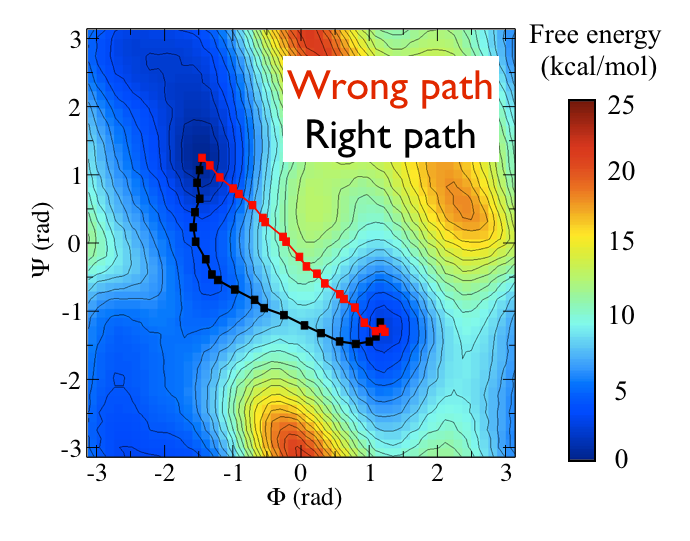
So, in this example we do a sort of "commmittor analysis" where we start shooting a number of free molecular dynamics from the saddle point located at \( \Phi=0 \) and \( \Psi=-1 \) and we want to see which way do they go. Intuitively, by assigning random velocities every time we should find part of the trajectories that move woward \( C_7eq \) and part that move towards \( C_7ax \).
I provided you with two directories, each containing a bash script script.sh whose core (it is a bit more complicated in practice...) consists in:
#
# set how many runs you want to do
#
ntests=50
for i in `seq 1 $ntests`
do
        #
        # assign a random velocity at each timestep by initializing the
        #
        sed s/SEED/$RANDOM/ md.mdp >newmd.mdp
        #
        # do the topology: this should write a topol.tpr
        #
        $GROMPP -c start.gro -p topol.top -f newmd.mdp
        $GROMACS_BIN/$MDRUN -plumed plumed.dat
        mv colvar colvar_$i
done
This runs 50 short MD runs (few hundreds steps) and just saves the colvar file into a labeled colvar file. In each mdrun plumed is used to plot the collective variables and it is something that reads like the follwing:
# Phi
t1: TORSION ATOMS=5,7,9,15
# Psi
t2: TORSION ATOMS=7,9,15,17
# The right path
p1: PATHMSD REFERENCE=right_path.dat LAMBDA=15100.
# The wrong path
p2: PATHMSD REFERENCE=wrong_path.dat  LAMBDA=8244.4
# Just a printout of all the stuff calculated so far
PRINT ARG=* STRIDE=2 FILE=colvar FMT=%12.8f
where I just want to plot \( \Phi \) , \( \Psi \) and the two path collective variables. Note that each path has a different LAMBDA parameters. Here the Ramachandran angles are plotted so you can realize which path is the system walking in a more confortable projection. This is of course fine in such a small system but whenever you have to deal with larger systems and control hundreds of CVs at the same time, I think that path collective variables produce a more intuituve description for what you want to do.
If you run the script simply with
pd@plumed:~> ./script.sh
then after a minute or so, you should have a directory which is full of colvar files. Let's revise together how the colvar file is formatted:
#! FIELDS time t1 t2 p1.sss p1.zzz p2.sss p2.zzz
#! SET min_t1 -pi
#! SET max_t1 pi
#! SET min_t2 -pi
#! SET max_t2 pi
 0.000000  -0.17752998  -1.01329788  13.87216908   0.00005492  12.00532256   0.00233905
 0.004000  -0.13370142  -1.10611136  13.87613508   0.00004823  12.03390658   0.00255806
 0.008000  -0.15633049  -1.14298481  13.88290617   0.00004511  12.07203319   0.00273764
 0.012000  -0.23856451  -1.12343958  13.89969608   0.00004267  12.12872544   0.00284883
...
In first column you have the time, then t1 ( \( \Phi \)) , then t2 ( \( \Psi \) ) and the path collective variables p1 and p2. Note that the action PATHMSD calculates both the progress along the path (p1.sss) and the distance from it (p1.zzz) . In PLUMED jargon, these are called "components". So a single Action (a line in plumed input) can calculate many components at the same time. This is not always the case: sometimes by default you have one component but specific flags may enable more components to be calculated (see DISTANCE for example). Note that the header (all the part of a colvar file that contains # as first character) is telling already what it inside the file and eventually also tells you if a variable is contained in boundaries (for example torsions, are periodic and their codomain is defined in -Pi and Pi ).
At the end of the script, you also have two additional scripts. One is named script_rama.gplt and the other is named script_path.gplt. They contain some gnuplot commands that are very handy to visualize all the colvar files without making you load one by one, that would be a pain.
Now, let's visualize the result from the wrong path directory. In order to do so, after having run the calculation, then do
pd@plumed:~>gnuplot
gnuplot> load "script_rama.gplt"
what you see is that all the trajectories join the reactant and the product state along the low free energy path depicted before.
Now if you try to load the same bunch of trajectories as a function of the progress along the path and the distance from the path in the case of the wrong path then simply do
gnuplot> load "script_path_wrong.gplt"
What do you see? A number of trajectories move from the middle towards the right bottom side at low distance from the path. In the middle of the progress along the path, you have higher distance. This is expected since the distance zero corresponds to a unlikely, highly-energetic path which is unlikely to occur. Differently, if you now do
gnuplot> load "script_path_right.gplt"
You see that the path, compared to what happened before, run much closer to small distance from the path. This means that the provided path is highlt resemblant and representative of what hapens in the reactive path.
Note that going at high distances can be also beneficial. It might help you to explore alternative paths that you have not explored before. But beware, the more you get far from the path, the more states are accessible, in a similar way as the fact that the surface of a sphere increase with its radius. The surface ramps up much faster than the radius therefore you have a lots of states there. This means also high entropy, so many systems actually tend to drift to high distances while, on the contrary, zero distance is never reached in practice (zero entropy system is impossible to reach at finite temperature). So you can see by yourself that this can be a big can of worms. In particular, my experience with path collective variables and biological systems tells me that most of time is hopeless to go to high distances to find new path in many cases (for example, in folding). While this is worth whenever you think that the paths are not too many (alternative routes in chemical reaction or enzymatic catalysis).
Very often it is asked how to format a set of pdb to be suitably used with path collective variables. Here are some tricks.
This section is actually set a bit foward but I included here for completeness now. It is recommended to be read after you have an introduction on Metadynamics and to well-tempered Metadynamics in particular. Here I want to show a couple of concept together.
Let's go to the last problem. All comes from the derivative belfast-2-sder-eq. Whenever you have a point of phase space which is similar to one of the endpoint than one of the points in the center then you get a \( s(X) \) which is 1 or N (where N is the number of frames composing the path collective variable). In this case that exponential will dominate the others and you are left with a constant (since the derivative of RMSD is a constant since it is linear in space). This means that, no matter what happens here, you have small force. Additionally you have small motion in the CV space. You can move a lot in configuration space but if the closest point is one of the endpoint, your CV value will always be one of the endpoint itself. So, if you use a fixed width of your CV which you retrieve from a middle point in your path, this is not suitable at all at the endpoints where your CV flucutates much less. On the contrary if you pick the hills width by making a free dynamics on the end states you might pick some sigmas that are smaller than what you might use in the middle of the path. This might give a rough free energy profile and definitely more time to converge. A possible solution is to use the adaptive gaussian width scheme. In this scheme you adapt the hills to their fluctuation in time. You find more details in [11] Additionally you also adopt a non spherical shape taking into account variable correlation. So in this scheme you do not have to fix one sigma per variable sigma, but just the time in which you calculate this correlation (another possibility is to calculate it from the compression of phase space but will not be covered here). The input of metadynamics might become something like this
t1: TORSION ATOMS=5,7,9,15
t2: TORSION ATOMS=7,9,15,17
p1: PATHMSD REFERENCE=right_path.dat LAMBDA=15100.
p2: PATHMSD REFERENCE=wrong_path.dat  LAMBDA=8244.4
#
# do a metadynamics on the right path, use adaptive hills whose decay time is 125 steps (250 fs)
# and rather standard WT parameters
#
meta: METAD ARG=p1.sss,p1.zzz  ADAPTIVE=DIFF SIGMA=125 HEIGHT=2.4 TEMP=300 BIASFACTOR=12 PACE=125
PRINT ARG=* STRIDE=10 FILE=colvar FMT=%12.8f
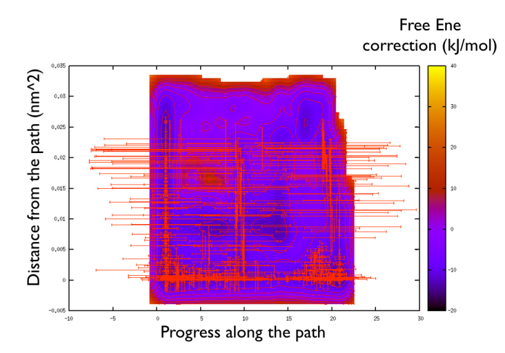
You can find this example in the directory BIASED_DYNAMICS. After you run for a while it is interesting to have a feeling for the change in shape of the hills. That you can do with
pd@plumed:~> gnuplot
gnuplot>  p "<head -400 HILLS" u 2:3:4:5 w xyer
that plots the hills in the progress along the path and the distance from the path and add an error bar which reflects the diagonal width of the flexible hills for the first 400 hills (Hey note the funny trick in gnuplot in which you can manipulate the data like in a bash script directly in gnuplot. That's very handy!).
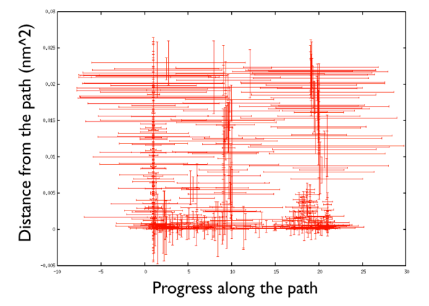
There are a number of things to observe: first that the path explores high distance since the metadynamics is working also in the distance from the path thus accessing the paths that were not explored before, namely the one that goes from the upper left corner of the ramachandran plot and the one that passes through the lower left corner. So in this way one can also explore other paths. Additionally you can see that the hills are changing size rather considerably. This helps the system to travel faster since at each time you use something that has a nonzero gradient and your forces act on your system in an effective way. Another point is that you can see broad hills covering places which you have not visited in practice. For example you see that hills extend so wide to cover point that have negative progress along the path, which is impossible by using the present definition of the progress along the path. This introduced a problem in calculating the free energy. You actually have to correct for the point that you visited in reality.
You can actually use sum_hills to this purpose in a two-step procedure. First you calculate the negative bias on a given range:
pd@plumed:~> plumed sum_hills --hills HILLS --negbias --outfile negative_bias.dat --bin 100,100 --min -5,-0.005 --max 25,0.05
and then calculate the correction. You can use the same hills file for that purpose. The initial transient time should not matter if your simulation is long enough to see many recrossing and, secondly, you should check that the hills heigh in the welltempered are small compared to the beginning.
pd@plumed:~> plumed sum_hills --histo HILLS --bin 100,100 --min -5,-0.005 --max 25,0.05 --kt 2.5 --sigma 0.5,0.001 --outhisto correction.dat
Note that in the correction you should assign a sigma, that is a "trust radius" in which you think that whenever you have a point somewhere, there in the neighborhood you assign a bin (it is done with Gaussian in reality, but this does not matter much). This is the important point that compenstates for the issues you might encounter putting excessive large hills in places that you have not visited. It is nice to have a look to the correction and compare with the hills in the same range.
gnuplot> set pm3d
gnuplot> spl "correction.dat" u 1:2:3 w l
gnuplot> set contour
gnuplot> set cntrp lev incremental -20,4.,1000.
gnuplot> set view map
gnuplot> unset clabel
gnuplot> replot
You might notice that there are no contour in the unrealistic range, this means that the free energy correction is impossible to calculate since it is too high (see Fig. belfast-2-metadpath-correction-fig ).
Now the last thing that one has to do to have the most plausible free energy landscape is to sum both the correction and the negative bias produced. This can be easily done in gnuplot as follows:
gnuplot> set pm3d
gnuplot> spl "<paste negative_bias.dat correction.dat " u 1:2:($3+$8) w pm3d
gnuplot> set view map
gnuplot> unset key
gnuplot> set xr [-2:23]
gnuplot> set contour
gnuplot> unset clabel
gnuplot> set cbrange [-140:-30]
gnuplot> set cntrp lev incr -140,6,-30
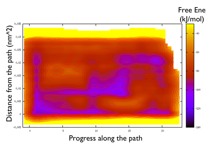
So now we can comment a bit on the free energy surface obtained and note that there is a free energy path that connects the two endpoints and runs very close to zero distance from the path. This means that our input path is actually resemblant of what is really happening in the system. Additionally you can see that there are many comparable routes different from the straight path. Can you make a sense of it just by looking at the free energy on the Ramachandran plot?
 1.8.10
