 |
|
|
| |
|
|
The aim of this tutorial is to introduce the users to the use of Bias-Exchange Metadynamics. We will go through the writing of the input files for BEMETA for a simple case of three peptide and we will use METAGUI to to analyse them. We will compare the results of WT-BEMETA and STANDARD-BEMETA with four independent runs on the four Collective Variables. Finally we will use a simplified version of BEMETA that is Multiple Walkers Metadynamics.
Once this tutorial is completed students will:
The tarball for this project contains the following files:
In all variants of metadynamics the free-energy landscape of the system is reconstructed by gradually filling the local minima with gaussian hills. The dimensionality of the landscape is equal to the number of CVs which are biased, and typically a number of CVs smaller than three is employed. The reason for this is that qualitatively, if the CVs are not correlated among them, the simulation time required to fill the free-energy landscape grows exponentially with the number of CVs. This limitation can be severe when studying complex transformations or reactions in which more than say three relevant CVs can be identified.
A possible technique to overcome this limitation is parallel-tempering metadynamics, Belfast tutorial: Replica exchange I. A different solution is performing a bias-exchange simulation: in this approach a relatively large number N of CVs is chosen to describe the possible transformations of the system (e.g., to study the conformations of a peptide one may consider all the dihedral angles between amino acids). Then, N metadynamics simulations (replicas) are run on the same system at the same temperature, biasing a different CV in each replica.
Normally, in these conditions, each bias profile would converge very slowly to the equilibrium free-energy, due to hysteresis. Instead, in the bias-exchange approach every fixed number of steps (say 10,000) an exchange is attempted between a randomly selected pair of replicas \( a \) and \( b \). The probability to accept the exchange is given by a Metropolis rule:
\[ \min\left( 1, \exp \left[ \beta ( V_G^a(x^a,t)+V_G^b(x^b,t)-V_G^a(x^b,t)-V_G^b(x^a,t) ) \right] \right) \]
where \( x^{a} \) and \( x^{b} \) are the coordinates of replicas \(a \) and \( b \) and \( V_{G}^{a(b)}\left(x,t\right) \) is the metadynamics potential acting on the replica \( a \)( \( b \)). Each trajectory evolves through the high dimensional free energy landscape in the space of the CVs sequentially biased by different metadynamics potentials acting on one CV at each time. The results of the simulation are N one-dimensional projections of the free energy.
In the following example, a bias-exchange simulation is performed on a VIL peptide (zwitterionic form, in vacuum with \( \epsilon=80 \), force field amber03), using the four backbone dihedral angles as CVs.
Four replicas of the system are employed, each one biased on a different CV, thus four similar Plumed input files are prepared as follows:
MOLINFO STRUCTURE=VIL.pdb
RANDOM_EXCHANGES

cv1: TORSION ATOMS=@psi-1
cv2: TORSION ATOMS=@phi-2
cv3: TORSION ATOMS=@psi-2
cv4: TORSION ATOMS=@phi-3
NOTE:
INCLUDE FILE=plumed-common.dat
be: METAD ARG=cv1 HEIGHT=0.2 SIGMA=0.2 PACE=100 GRID_MIN=-pi GRID_MAX=pi
PRINT ARG=cv1,cv2,cv3,cv4 STRIDE=1000 FILE=COLVAR
NOTE:
PRINT ARG=cv1,be.bias STRIDE=xxx FILE=BIAS
The four replicas start from the same GROMACS topology file replicated four times: topol0.tpr, topol1.tpr, topol2.tpr, topol3.tpr. Finally, GROMACS is launched as a parallel run on 4 cores, with one replica per core, with the command
mpirun -np 4 gmx_mpi mdrun -s topol -plumed plumed -multi 4 -replex 2000 >& log &
where -replex 2000 indicates that every 2000 molecular-dynamics steps all replicas are randomly paired (e.g. 0-2 and 1-3) and exchanges are attempted between each pair (as printed in the GROMACS *.log files).
The same simulation can be run using WELLTEMPERED metadynamics.
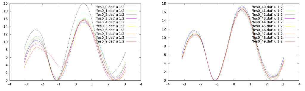
In the resources for this tutorial you can find the results for a 40ns long Well-Tempered Bias Exchange simulation. First of all we can try to assess the convergence of the simulations by looking at the profiles. In the "convergence" folder there is a script that calculates the free energy from the HILLS.0 file at incresing simulation lengths (i.e. every more 0.8 ns of simulation). The scripts also generate two measures of the evolution of the profiles in time:
From both plots one can deduce that after 8 ns the profiles don't change significantly thus suggesting that averaging over the range 8-40ns should result in a accurate profile (we will test this using metagui). Another test is that of looking at the fluctuations of the profiles in a time window instead of looking at successive profiles:
In principle Bias-Exchange Metadynamics can give as a results only N 1D free energy profiles. But the information contained in all the replicas can be used to recover multidensional free energy surfaces in >=N dimensions. A simple way to perform this analysis is to use METAGUI. METAGUI performs the following operations:
METAGUI (Biarnes et. al) is a plugin for VMD that implements the approch developed by Marinelli et. al 2009. It can be downloaded from the PLUMED website.
In order for the colvar and hills file to be compatible with METAGUI their header must be formatted as following:
COLVAR.#:
#! FIELDS time cv1 cv2 cv3 cv4
#! ACTIVE 1 1 A
#! ..
...
NOTE:
COLVAR.0:
#! FIELDS time cv1 cv2 cv3
#! ACTIVE 1 1 A
#! ..
...
COLVAR.1:
#! FIELDS time cv1 cv2 cv3
#! ACTIVE 1 2 B
#! ..
...
COLVAR.2:
#! FIELDS time cv1 cv2 cv3
#! ACTIVE 1 2 C
#! ..
...
COLVAR.3:
#! FIELDS time cv1 cv2 cv3
#! ACTIVE 0
#! ..
...
In the above case Replica 0 biases cv1; replicas 1 and 2 biases cv2 while replica 3 is a neutral (unbiased) replica. cv3 is unbiased in all the replicas.
The ACTIVE keyword must be the FIRST LINE in the HILLS.# files:
HILLS.#:
#! ACTIVE 1 1 A
#! FIELDS time cv1 sigma_cv1 height biasf
#! ..
...
The above notes hold for the HILLS files as well. In the folder metagui the script check_for_metagui.sh checks if the header of your file is compatible with METAGUI, but remember that this is not enough! Synchronisation of COLVAR and trajectory files is also needed. HILLS files can be written with a different frequency but times must be consistent.
NOTE: It is important to copy HILLS files in the metagui folder.
./check_for_metagui.sh ../COLVAR.0
will tell you that the ACTIVE keyword is missing, you need to modify all the header BEFORE proceeding with the tutorial!!
In the metagui folder there is a metagui.input file:
WHAM_EXE        wham_bemeta.x
BASINS_EXE      kinetic_basins.x
KT 2.4900
HILLS_FILE   HILLS.0
HILLS_FILE   HILLS.1
HILLS_FILE   HILLS.2
HILLS_FILE   HILLS.3
GRO_FILE     VIL.pdb
COLVAR_FILE COLVAR.0 ../traj0.xtc "psi-1"
COLVAR_FILE COLVAR.1 ../traj1.xtc "phi-2"
COLVAR_FILE COLVAR.2 ../traj2.xtc "psi-2"
COLVAR_FILE COLVAR.3 ../traj3.xtc "phi-3"
TRAJ_SKIP 10
CVGRID 1  -3.1415 3.1415 15 PERIODIC
CVGRID 2  -3.1415 3.1415 15 PERIODIC
CVGRID 3  -3.1415 3.1415 15 PERIODIC
CVGRID 4  -3.1415 3.1415 15 PERIODIC
ACTIVE 4 1 2 3 4
T_CLUSTER 0.
T_FILL    8000.
DELTA 4
GCORR 1
TR_N_EXP 5
where are defined the temperature in energy units, the place where to find COLVAR, HILLS and trajectory files. A reference gro or pdb file is needed to load the trajectories. The definition of the ranges and the number of bins for the available collective variables.
Now let's start with the analysis:
In order to visualise the microstate it is convenient to align all the structures using the VMD RMSD Trajectory tool that can be found in Extensions->Analysis.
One or more microstates can be visualised by selecting them and clicking show.
You can sort the microstates using the column name tabs, for example by clicking on size the microstates will be ordered from the larger to the smaller. If you look at the largest one it is possible to observe that by using the four selected collective variables the backbone conformation of the peptide is well defined while the sidechains can populate different rotameric states.
The equilibrium time in the analysis panel should be such that by averaging over the two halves of the remind of the simulation the profiles are the same (i.e the profile averaged between Teq and Teq+(Ttot-Teq)/2 should be the same of that averaged from Teq+(Ttot-Teq)/2 and Ttot). By clicking on COMPUTE FREE ENERGIES, the program will first generate the 1D free energy profiles from the HILLS files and then run the WHAM analysis on the microstates. Once the analysis is done it is possible to visually check the convergence of the 1D profiles one by one by clicking on the K bottons next to the HILLS.# files. The BLUE and the RED profiles are the two profiles just defined, while the GREEN is the average of the two. Now it is possible for example to sort the microstates as a function of the free energy and save them by dumping the structures for further analysis.
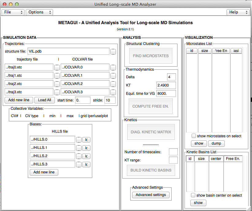
If you look in the metagui folder you will see a lot of files, some of them can be very usefull:
metagui/MICROSTATES: is the content of the microstates list table metagui/WHAM_RUN/VG_HILLS.#: are the opposite of the free energies calculated from the hills files metagui/WHAM_RUN/*.gnp: are gnuplot input files to plot the VG_HILLS.# files (i.e. gnuplot -> load "convergence..") metagui/WHAM_RUN/FES: is the result of the WHAM, for each cluster there is its free energy and the error estimate from WHAM
gnuplot> plot [0:40]'FES' u 2:3
plots the microstate error in the free energy estimate as a function of the microstates free energy. Finally in the folder metagui/FES there is script to integrate the multidimensional free energy contained in the MICROSTATES files to a 2D FES as a function of two of the used CV. To use it is enough to copy the MICROSTATES file in FES:
cp MICROSTATES FES/FES.4D
and edit the script to select the two columns of MICROSTATES on which show the integrated FES.
Multiple Walker metadynamics is the simplest way to parallelise a MetaD calculation: multiple simulation of the same system are run in parallel using metadynamics on the same set of collective variables. The deposited bias is shared among the replicas in such a way that the history dependent potential depends on the whole history.
We can use the same common input file defined above and then we can define four metadynamics bias in a similar way of what was done above for bias-exchange but now all the biases are defined on the same collective variables:
plumed.#.dat
INCLUDE FILE=plumed-common.dat

METAD ...
LABEL=mw
ARG=cv2,cv3
SIGMA=0.3,0.3
HEIGHT=0.2
PACE=100
BIASFACTOR=8
GRID_MIN=-pi,-pi
GRID_MAX=pi,pi
WALKERS_MPI
... METAD

PRINT ARG=cv1,cv2,cv3,cv4 STRIDE=1000 FILE=COLVAR
and the simulation can be run in a similar way without doing exchanges:
mpirun -np 4 gmx_mpi mdrun -s topol -plumed plumed -multi 4 >& log &
alternatively Multiple Walkers can be run as independent simulations sharing via the file system the biasing potential, this is usefull because it provides a parallelisation that does not need a parallel code. In this case the walkers read with a given frequency the gaussians deposited by the others and add them to their own METAD.
This tutorial is freely inspired to the work of Biarnes et al.
More materials can be found in
 1.8.14