 |
|
|
| |
|
|
The aim of this Masterclass is to introduce users to the PLUMED syntax and to illustrate how PLUMED can be used to analyze pre-existing molecular dynamics trajectories.
Once this Masterclass is completed, users will be able to:
We will use conda to install all the software needed in this Masterclass:
First, make sure conda is installed by typing:
conda
If the command is not found, please refer to these instructions to install conda on your machine. Alternatively, if you use the Homebrew package manager, you can install conda with:
brew install --cask anaconda
# add this line to your .bashrc
export PATH="/usr/local/anaconda3/bin:$PATH"
Now we can create a conda environment for the PLUMED Masterclass:
conda create --name plumed-masterclass
and activate it with:
conda activate plumed-masterclass
Finally, we can proceed with the installation of the required software:
conda install -c conda-forge plumed py-plumed numpy pandas matplotlib notebook mdtraj mdanalysis git
plumed-masterclass environment every time you open a new terminal/shell.PLUMED is a library that can be incorporated into many molecular dynamics (MD) codes by adding a relatively simple and well documented interface. Once it is incorporated you can use PLUMED to perform on-the-fly a variety of different analyses and to bias the sampling in MD simulations. Additionally, PLUMED can be used as a standalone code for analyzing trajectories. If you want to use the code in this way, you can run the PLUMED executable by issuing the command:
plumed <instructions>
Let's start by getting a feel for the range of calculations that PLUMED can do. Issue the following command now:
plumed --help
The output of this command is the list of Command Line Tools included in PLUMED. Among these, there are commands that allow you to patch an MD code, postprocess metadynamics simulations, and build the manual. In this class we will use PLUMED to analyze trajectories. In order to do so, we will learn how to use the driver command line tool. Let's look at the options of PLUMED driver by issuing the following command:
plumed driver --help
As you can see we can do a number of things with driver. For all of these options, however, we are going to need to write a PLUMED input file.
The data needed to complete the exercises of this Masterclass can be found on GitHub. You can clone this repository locally on your machine using the following command:
git clone https://github.com/plumed/masterclass-21-1.git
The MD trajectory that we will analyze can be found in the folder called data:
5-HT1B.pdb: reference conformation of the 5-HT1B receptor with the serotonin ligand.5-HT1B.xtc: trajectory of the 5-HT1B receptor with the serotonin ligand.A Jupyter notebook to be used as template for the analysis of the PLUMED output can be found in the folder called notebooks. In this directory, you will also find the complete solution to all exercises in the notebook solution.ipynb.
Please note that:
To keep things clean, it is recommended to run each exercise in a separate sub-directory (i.e. Exercise-1, Exercise-2, ...), which you can create inside the root directory masterclass-21-1.
The main goal of PLUMED is to compute collective variables (or CVs), which are complex descriptors of the system that can be used to describe the conformational change of a protein or a chemical reaction. This can be done either on-the-fly during a molecular dynamics simulations or a posteriori on a pre-calculated trajectory using PLUMED as a post-processing tool. In both cases, you should create an input file with a specific PLUMED syntax. Have a look at the sample input file below:
# Compute distance between atoms 1 and 10. # Atoms are ordered as in the trajectory files and their numbering starts from 1. # The distance is called "d" for future reference. d: DISTANCEATOMS=1,10 # Compute the torsional angle between atoms 1, 10, 20, and 30. # The angle is called "phi1" for future reference. phi1: TORSIONthe pair of atom that we are calculating the distance between.ATOMS=1,10,20,30 # The same CV defined above can be split into multiple lines # The angle is called "phi2" for future reference. phi2: TORSION ...the four atoms involved in the torsional angleATOMS=1,10,20,30 ... # Print "d" on a file named "COLVAR1" every 10 steps. PRINTthe four atoms involved in the torsional angleARG=dthe input for this action is the scalar output from one or more other actions.FILE=COLVAR1the name of the file on which to output these quantitiesSTRIDE=10 # Print "phi1" and "phi2" on another file named "COLVAR2" every 100 steps. PRINTcompulsory keyword ( default=1 ) the frequency with which the quantities of interest should be outputARG=phi1,phi2the input for this action is the scalar output from one or more other actions.FILE=COLVAR2the name of the file on which to output these quantitiesSTRIDE=100compulsory keyword ( default=1 ) the frequency with which the quantities of interest should be output
In the input file above, each line defines a so-called action. In this simple example, actions are used to compute a distance, a dihedral angle, or print some values on a file. Each action supports a number of keywords, whose value is specified. Action names are highlighted in green and, by clicking on them, you can go to the corresponding page in the manual that contains a detailed description of each keyword. Actions that support the keyword STRIDE are those that determine how frequently things are done. Notice that the default value for STRIDE is always 1. In the example above, omitting STRIDE keywords the corresponding COLVAR files would have been written for every frame of the analyzed trajectory. All the other actions in the example above, i.e. DISTANCE and TORSION, do not support the STRIDE keyword and are only calculated when requested. That is, d will be computed every 10 frames, and phi1 and phi2 every 100 frames.
Variables should be given a name (in the example above, d, phi1, and phi2), which is then used to refer to these variables in subsequent actions, such as the PRINT command. A lists of atoms should be provided as comma separated numbers, with no space.
You can find more information on the PLUMED syntax at Getting Started page of the manual. The complete documentation for all the supported collective variables can be found at the Collective Variables page.
By default the PLUMED inputs and outputs quantities in the following units:
If you want to change these units, you can do this using the UNITS keyword.
In this exercise, we will learn how to compute and print collective variables on a pre-calculated MD trajectory. To analyze the trajectory provided here, we will:
plumed.dat);Notice that you can also visualize trajectories with VMD (always a good idea!). For example, the trajectory 5-HT1B.xtc can be visualized with the command:
vmd 5-HT1B.pdb 5-HT1B.xtc
When you try this, you will notice that this trajectory is discontinuous due to PBCs. We need to keep this in mind in our analysis.
Let's now prepare a PLUMED input file to calculate:
The first 40 residues of the 5-HT1B receptor correspond to an extracellular flexible loop of which we want to characterize the dynamics during our MD simulation. Below you can find a sample plumed.dat file that you can use as a template. Whenever you see an highlighted FILL string, be careful because this is a string that you must replace. To retrieve the atom indexes that you need to include in the input file, you can have a look at 5-HT1B.pdb. The atoms indexes are contained in the second column. Keep in mind that numbering scheme in PLUMED starts from 1.
# Compute gyration radius on CA atoms of the first 40 N-terminal residues: r: GYRATIONATOMS=__FILL__ # Compute distance between CA atoms of residues 1 and 40 d: DISTANCEthe group of atoms that you are calculating the Gyration Tensor for.ATOMS=__FILL__ # Print the two collective variables on COLVAR file every step PRINTthe pair of atom that we are calculating the distance between.ARG=__FILL__the input for this action is the scalar output from one or more other actions.FILE=COLVARthe name of the file on which to output these quantitiesSTRIDE=__FILL__compulsory keyword ( default=1 ) the frequency with which the quantities of interest should be output
Once your plumed.dat file is complete, you can run the PLUMED driver as follows:
plumed driver --plumed plumed.dat --mf_xtc 5-HT1B.xtc
Scroll in your terminal to read the PLUMED log. As you can see, PLUMED gives a lot of feedback about the input that it is reading and the actions that it will execute. Please take your time to inspect the log file and check if PLUMED is actually doing what you intend to do.
The command above will create a COLVAR file. The first lines should be identical to these ones:
#! FIELDS time r d
 0.000000 1.271069 2.782998
 1.000000 1.263125 2.388697
 2.000000 1.348965 2.606062
 3.000000 1.291011 2.204363
 4.000000 1.280714 2.411836
 5.000000 1.257692 2.334839
Notice that the first line informs you about the content of each column.
In case you obtain different numbers, check your input, you might have made some mistakes!
This COLVAR file can be analyzed using the Jupyter notebook plumed-pandas.ipynb provided in the folder notebooks. You can use the following command to open the notebook:
jupyter notebook plumed-pandas.ipynb
This notebook allows you to import the COLVAR file produced by PLUMED and to generate the desired figures using the matplotlib library:
What can you deduce about the dynamics of this region of the 5-HT1B receptors? Are the two CVs both providing useful information or are they quite correlated? To answer to the latter question, you can inspect the plot of one CV against the other.
PLUMED provides some shortcuts to select atoms with specific properties. To use this feature, you should specify the MOLINFO action along with a reference PDB file. This command is used to provide information on the molecules that are present in your system.
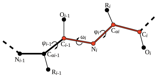
Let's try to use this functionality to calculate the backbone dihedral angle \( \phi \) (phi) of residue 2 of the 5-HT1B receptor. This CV is defined by the action TORSION and a set of 4 atoms. For residue i, the dihedral \( \phi \) is defined by these atoms: C(i-1),N(i),CA(i),C(i) (see Fig. masterclass-21-1-dih-fig).
After consulting the manual and inspecting 5-HT1B.pdb, let's define the dihedral angle \( \phi \) of residue 2 in two different ways:
t1).t2);# Activate MOLINFO functionalities MOLINFOSTRUCTURE=__FILL__ # Define the dihedral phi of residue 2 as an explicit list of 4 atoms t1: TORSIONcompulsory keyword a file in pdb format containing a reference structure.ATOMS=__FILL__ # Define the same dihedral using MOLINFO shortcuts t2: TORSIONthe four atoms involved in the torsional angleATOMS=__FILL__ # Print the two collective variables on COLVAR file every step PRINTthe four atoms involved in the torsional angleARG=__FILL__the input for this action is the scalar output from one or more other actions.FILE=COLVARthe name of the file on which to output these quantitiesSTRIDE=__FILL__compulsory keyword ( default=1 ) the frequency with which the quantities of interest should be output
After completing the PLUMED input file above, let's use it to analyze the trajectory 5-HT1B.xtc using the driver tool:
plumed driver --plumed plumed.dat --mf_xtc 5-HT1B.xtc
You can modify the Jupyter notebook used in Exercise 1: Computing and printing simple collective variables to visualize the trajectory of the two CVs calculated with the PLUMED input file above and written in the COLVAR file. If you executed this exercise correctly, these two trajectories should be identical.
As a second example of MOLINFO capabilities, we will use the advanced atom selection tools provided by the MDAnalysis and MDTraj libraries. Let's redo Exercise 1: Computing and printing simple collective variables, this time using MOLINFO shortcuts to select CA atoms. You need to complete the following template PLUMED input file using the appropriate selection syntax for the corresponding library used. Please consult the MDAnalysis and MDTraj documentations if you are not familiar with these libraries and their syntax.
# Activate MOLINFO functionalities MOLINFOSTRUCTURE=__FILL__ # To use MDAnalysis selection tools: r1: GYRATIONcompulsory keyword a file in pdb format containing a reference structure.ATOMS={@mda:{resid __FILL__ and name __FILL__}} d1: DISTANCEthe group of atoms that you are calculating the Gyration Tensor for.ATOMS={@mda:{resid __FILL__ and name __FILL__}} # To use MDTraj selection tools: r2: GYRATIONthe pair of atom that we are calculating the distance between.ATOMS={@mdt:{resid __FILL__ and name __FILL__}} d2: DISTANCEthe group of atoms that you are calculating the Gyration Tensor for.ATOMS={@mdt:{resid __FILL__ and name __FILL__}} # Print all the collective variables on COLVAR file every step PRINTthe pair of atom that we are calculating the distance between.ARG=__FILL__the input for this action is the scalar output from one or more other actions.FILE=COLVARthe name of the file on which to output these quantitiesSTRIDE=__FILL__compulsory keyword ( default=1 ) the frequency with which the quantities of interest should be output
Now, you can compare the COLVAR file obtained with the one of Exercise 1: Computing and printing simple collective variables: they should be identical!
Sometimes, when calculating a CV, you may not want to use the positions of a number of atoms directly. Instead you may want to define a virtual atom whose position is generated based on the positions of a collection of other atoms. For example you might want to use the center of mass (COM) or the geometric center (CENTER) of a group of atoms.
In this exercise, you will learn how to specify virtual atoms and later use them to define a CV. The objective is to calculate the distances between the geometric center of the serotonin ligand (indicated as residue LIG in 5-HT1B.pdb) and the geometric centers of the two glycans located at position N24 and N32. Glycans are carbohydrate-based polymers that are sometimes linked to certain protein aminoacids. If you examine 5-HT1B.pdb, you will find the two glycans defined after the end of the protein, i.e. after residue SER-390. These two glycans have different length:
Let's complete the PLUMED input file below. You can use the advanced selection tools learned in Exercise 2: Mastering advanced selection tools to specify the atoms belonging to the ligand and to the two glycans:
# Geometric center of the ligand lig: CENTERATOMS=__FILL__ # Geometric center of the first glycan g1: CENTERthe list of atoms which are involved the virtual atom's definition.ATOMS=__FILL__ # Geometric center of the second glycan g2: CENTERthe list of atoms which are involved the virtual atom's definition.ATOMS=__FILL__ # Distance between ligand and first glycan d1: DISTANCEthe list of atoms which are involved the virtual atom's definition.ATOMS=__FILL__ # Distance between ligand and second glycan d2: DISTANCEthe pair of atom that we are calculating the distance between.ATOMS=__FILL__ # Print the two distances on COLVAR file every step PRINTthe pair of atom that we are calculating the distance between.ARG=__FILL__the input for this action is the scalar output from one or more other actions.FILE=COLVARthe name of the file on which to output these quantitiesSTRIDE=__FILL__compulsory keyword ( default=1 ) the frequency with which the quantities of interest should be output
Once you have prepared a PLUMED input file containing the above instructions, you can execute it on the trajectory 5-HT1B.xtc by making use of the following command:
plumed driver --mf_xtc 5-HT1B.xtc --plumed plumed.dat
Let's now analyze the output of the calculation by plotting the time series of the two CVs. Can you say if the ligand is overall staying closer to the first or second glycan?
As mentioned above, 5-HT1B.xtc is the raw trajectory generated by the GROMACS MD code. Therefore, it typically presents discontinuities due to PBCs. Many of the CVs used so far, such as CENTER or DISTANCE, take care of these discontinuities automatically. However, other CVs need a special command, called WHOLEMOLECULES, to fix PBCs discontinuities before the calculation of the CV. In this exercise, you will learn how to use this action.
We have seen that the first 40 N-terminal residues of the 5-HT1B receptor are quite flexibile. In this exercise, we want to estimate the secondary structure content (alpha-helix and beta-sheet) of this fragment during the course of the MD simulations. In order to do so, we can use the following 3 CVs:
Let's first try to complete the following PLUMED input file:
# Activate MOLINFO functionalities MOLINFO __FILL__ # make the first 40 N-terminal residues whole WHOLEMOLECULES __FILL__ # alpha-helix content of residues 1-40 h: ALPHARMSD __FILL__TYPE=OPTIMAL # parallel beta-sheet content of residues 1-40 pb: PARABETARMSD __FILL__compulsory keyword ( default=DRMSD ) the manner in which RMSD alignment is performed.TYPE=OPTIMAL # antiparallel beta sheet-content of residues 1-40 ab: ANTIBETARMSD __FILL__compulsory keyword ( default=DRMSD ) the manner in which RMSD alignment is performed.TYPE=OPTIMAL # now we create a new CV that sums parallel and antiparallel beta-sheet contents b: COMBINE __FILL__compulsory keyword ( default=DRMSD ) the manner in which RMSD alignment is performed.PERIODIC=NO # Print the alpha-helical content and the *total* beta-sheet content on COLVAR file every step PRINT __FILL__compulsory keyword if the output of your function is periodic then you should specify the periodicity of the function.
and use it to analyze the trajectory 5-HT1B.xtc. Can you say if the first 40 N-terminal residues tend to populate more alpha-helical or beta-sheet conformations?
As previously mentioned, the first 40 N-terminal residues of the 5-HT1B receptor are quite flexible, while the rest of the protein remains more stable during the course of the simulation. In this exercise, you will learn how to use RMSD to measure deviations from a reference structure. To use this CV, you need to keep in mind that you must specify in the PLUMED input a PDB file in which you mark the atoms that you want to use to:
Keep in mind that these two sets of atoms might be different! In fact, the objective of this exercise is to calculate:
To create the two PDB files needed to define the two RMSD CVs, you can start from the provided PDB file 5-HT1B.pdb. Please consult the manual at the RMSD page, in order to:
TYPE=OPTIMAL);After analyzing 5-HT1B.xtc with the driver tool, can you say which part of the receptor is more flexible and deviates more from the starting conformation during the course of the simulation?
In this exercise, we will learn how to align a MD trajectory to a reference conformation, after fixing possible discontinuities due to PBCs. The goal is to compute the vertical position of the serotonin ligand with respect to the lipid bilayer. In the simulations of membrane proteins, typically the initial conformation is oriented so that the lipid bilayer is parallel to the xy plane (look for example at 5-HT1B.pdb). Therefore, initially one could use for example the coordinate z of the geometric center of the ligand to measure how far it is from the membrane bilayer. However, during the simulation:
therefore one could not use an absolute position to keep track of the location of the ligand. To solve this problem, there are several PLUMED actions that can be used to make sure the system is not broken by PBCs, to re-align it to a reference conformation, and thus to use absolute positions safely.
To complete this exercise, the users will need to make heavy use of the PLUMED manual to prepare the input file on their own. In the following, some suggestions will be given:
GROUPBY option;5-HT1B.pdb, you can use FIT_TO_TEMPLATE;NOPBC;z component of the POSITION CV.You can check that your PLUMED input file is correct in two ways. First, you can print out the conformations of the system after the transformations done by WHOLEMOLECULES, WRAPAROUND, and FIT_TO_TEMPLATE by modifying your input file as follows:
# Activate MOLINFO functionalities MOLINFOSTRUCTURE=__FILL__ # Here put your PLUMED input file # # # Write coordinates of all the atoms to file after PLUMED transformations DUMPATOMScompulsory keyword a file in pdb format containing a reference structure.FILE=5-HT1B_aligned.grocompulsory keyword file on which to output coordinates; extension is automatically detectedATOMS=__FILL__the atom indices whose positions you would like to print out.
Now, you can visualize the 5-HT1B_aligned.gro file using VMD. Second, if you inspect the time series of your CV, this should be a continuous trajectory that spans the range from 9 nm to 18 nm.
In this last exercise, we want to determine the propensity of the serotonin ligand to bind the first 40 N-terminal flexible residues of the 5-HT1B receptor and if there are hot-spots where binding is more favorite. In order to answer to these questions, the user will:
gro file, after fixing PBCs as in Exercise 6: Aligning conformations to a template;gro file, after fixing PBCs.To solve this exercise, no template PLUMED input file nor any indication of the procedure to follow will be given. The users should only keep in mind that:
 1.8.17