 |
|
|
| |
|
|
In this Masterclass, we will discuss how to report the results from molecular simulations.
We will emphasize that any result that we get from any simulation is a random variable. To make the result reproducible, we must characterize the distribution that has been sampled. It is not sufficient to report the averages.
Once you have completed this Masterclass you will be able to:
If you have not yet set up PLUMED, you can find information about installing it in the section Setting up the software of PLUMED Masterclass 21.1: PLUMED syntax and analysis. Please ensure that you have setup PLUMED on your machine before starting the exercises.
The data needed to execute the exercises of this Masterclass can be found on GitHub. You can clone this repository locally on your machine using the following command:
git clone https://github.com/plumed/masterclass-21-2.git
The data you need is in the folder called data. You will find the following files in that folder:
uncorrelated_data: you will analyze this data set in the first six exercises that followcorrelated_data: you will analyze this data set in exercise 7weighted_data: you will analyze this data in exercise 8In exercise 9, you will pull everything together by generating a metadynamics trajectory. This exercise draws together all the ideas from exercises 1-8 by getting you to run a metadynamics simulation and extract the free energy surface. In the data folder, you will thus also find the following files, which are the input for the metadynamics simulation:
Notice that PLUMED input files have not been provided in the GitHub repository. You must prepare these input files yourself using the templates below.
We would recommend that you run each exercise in separate sub-directories inside the root directory masterclass-21-2.
PLUMED Masterclass 21.1: PLUMED syntax and analysis showed you how PLUMED can be used to calculate the value of a collective variables, \(s(\mathbf{x})\), from the positions of the atoms, \(\mathbf{x}\). You should also have seen that doing so allows you to describe the conformational changes or chemical reactions that have occured during your molecular dynamics trajectory. We will build on this idea in this tutorial by recalling that the values for collective variable we calculate for the frames of a constant-temperature molecular dynamics trajectory are samples from the probability distribution for the canonical (NVT) ensemble:
\[ P(s') = \frac{ \int \textrm{d}x \textrm{d}p \delta( s(x) - s') e^{-\frac{H(x,p)}{k_B T}} }{ \int \textrm{d}x\textrm{d}p e^{-\frac{H(x,p)}{k_B T}} } \]
where \(k_B\) is Boltzmann's constant, \(T\) is the temperature \(H(x,p)\) is the Hamiltonian and \(\delta\) is a Dirac delta function. Notice also that the integrals in the numerator and denominator are integrals over all of phase space. If \(N\) is the number of atoms in our system we must, therefore, integrate over each of the \(3N\) momentum ( \(p\)) and \(3N\) position ( \(x\)) coordinates when calculating these integrals.
It is only possible to calculate the integrals in the quotient above exactly for elementary physical systems. For more complex systems we thus assume that we can extract information on \(P(s')\) by sampling from this distribution multiple times (using molecular dynamics or Monte Carlo) and using the tools of statistics. Critically, however, any result we get from such simulations is a random variable. To make our results reproducible we thus need to characterize the distribution sampled in our simulation.
Reporting only the average value we get is not sufficient as any averages we take are random.
Links to background information on statistical mechanics and statistics are provided throughout this tutorial. You can complete the tutorial without looking at the information at these links. However, we hope that the information we have provided through these links will prove useful if you want to do a more in-depth study of the topic.
We will start our study of averaging by estimating the ensemble average of the CV. The ensemble average for \(s(x)\) is given by:
\[ \langle s \rangle = \frac{ \int \textrm{d}x \textrm{d}p s(x) e^{-\frac{H(x,p)}{k_B T}} }{ \int \textrm{d}x\textrm{d}p e^{-\frac{H(x,p)}{k_B T}} } \]
This equation is the same quotient that was introduced for \(P(s')\) in Background but with the Dirac delta replaced by \(s(x)\).
In statistics, the quantity known as the ensemble average in statistical mechanics is referred to as the expectation of the random variable's distribution. The expectation of a random variable is often esimated by taking multiple identical samples from the distribution, \(X_i\) and computing a sample mean as follows:
\[ \overline{X} = \frac{1}{N} \sum_{i=1}^N X_i \]
We can do the same with the data from our MD trajectory. We replace the \(X_i\) in the equation above with the CV values calculated for each of our trajectory frames.
To calculate averages using PLUMED, you can use the input file below. This input calculates averages for the data in the uncorrelated_data file you downloaded when you collected the GitHub repository.
data: READ FILEcompulsory keyword the name of the file from which to read these quantities =__FILL__ VALUEScompulsory keyword the values to read from the file =__FILL__ av: AVERAGE ARGthe input for this action is the scalar output from one or more other actions. =__FILL__ STRIDEcompulsory keyword ( default=1 ) the frequency with which the data should be collected and added to the quantity being averaged =1 PRINT ARGthe input for this action is the scalar output from one or more other actions. =av FILEthe name of the file on which to output these quantities =colvar
Copy the input to a file called plumed.dat, fill in the blanks and run the calculation by executing the following command:
> plumed driver --noatoms
The colvar file that is output by PLUMED contains the average computed value from progressively larger and larger numbers of CV values. You should thus be able to use the data in colvar to produce a graph that shows the average as a function of the number of variables it is computed from as shown below.
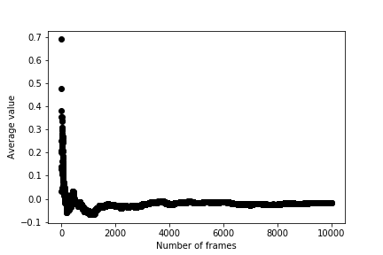
The fluctuations in the average get smaller as this quantity is computed from larger numbers of random variables. We say that the average thus converges to the ensemble average, which is zero for the graph above.
We can estimate the distribution for our CV, \(P(s')\) (see Background), by calculating a histogram. The histogram we obtain is a sample from a multinomial distribution so we can estimate parameters for the multinomial by using likelihood maximisation. Once we have the marginal distribution, \(P(s')\) we can then calculate the free energy, \(F(s')\) as a function of \(s(x)\) as \(F(s')\) is related to \(P(s')\) (see Background) by:
\[ F(s') = - k_B T \ln P(s') \]
If we estimate \(P(s')\) using likelihood maximisation we can thus get an estimate of the free energy surface. To estimate the free energy surface for the data in uncorrelated_data using PLUMED in this way we can use the input file:
# We use natural units here so that kBT is set to 1 UNITS NATURAL( default=off ) use natural units data: READ FILEcompulsory keyword the name of the file from which to read these quantities =__FILL__ VALUEScompulsory keyword the values to read from the file =__FILL__ hhh: HISTOGRAM ARGthe input for this action is the scalar output from one or more other actions. =__FILL__ STRIDEcompulsory keyword ( default=1 ) the frequency with which the data should be collected and added to the quantity being averaged =1 __FILL__ could not find this keyword =-4.5 __FILL__ could not find this keyword =4.5 __FILL__ could not find this keyword =100 __FILL__ could not find this keyword =DISCRETE fes: CONVERT_TO_FES GRIDcompulsory keyword the action that creates the input grid you would like to use =__FILL__ TEMPthe temperature at which you are operating =1 # This sets k_B T = 1 DUMPGRID GRIDcompulsory keyword the action that creates the grid you would like to output =__FILL__ FILEcompulsory keyword ( default=density ) the file on which to write the grid. =fes.dat
Copy this input to a file called plumed.dat, fill in the blanks so that you have a grid that runs from -4 to +4 with 100 bins. Run the calculation by executing the following command:
> plumed driver --noatoms
The --noatoms flag here is needed since plumed driver is commonly used to analize a trajectory of atomic coordinates, but here we are using it to directly analyze a collective variable.
You should see that the free energy curve for this data set looks like this:
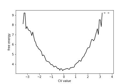
As you can see, there is a single minimum in this free energy surface.
Physical systems spend the majority of their time fluctuating around minima in the free energy landscape. Let's suppose that this minima is at \(\mu\) and lets use the Taylor series to write an expression for the free energy at \(s'\) as follows:
\[ F(s) = F(\mu) + F'(\mu)(s-\mu) + \frac{F''(\mu)(s-\mu)^2}{2!} + \dots + \frac{F^{(n)}(\mu)(s-\mu)^n}{n!} + \dots \]
In this expression \(F'(\mu)\), \(F''(\mu)\) and \(F^{(n)}(\mu)\) are the first, second and \(n\)th derivatives of the free energy at \(\mu\). We know there is a minimum at \(\mu\) so \(F'(\mu)=0\). If we truncate the expansion at second order we can, therefore, write:
\[ F(s) \approx F(\mu) + \frac{F''(\mu)(s-\mu)^2}{2} \]
We now recall that \(F(s) = - k_B T \ln P(s')\) and thus write:
\[ P(s) = \exp\left( -\frac{F(s)}{k_B T} \right) \approx \exp\left( -\frac{F(\mu) + \frac{F''(\mu)(s-\mu)^2}{2} }{k_B T} \right) = \exp\left( -\frac{F(\mu)}{k_B T} \right)\exp\left( - \frac{F''(\mu)(s-\mu)^2}{2k_B T} \right) \]
The first term in the final product here is a constant that does not depend on \(s\), while the second is a Gaussian centered on \(\mu\) with \(\sigma^2 = \frac{k_B T}{F''(\mu)}\).
We can assume that the constant term in the product above normalizes the distribution. The derivation above, therefore, suggests that our CV values are all samples from a normal distribution. We thus no longer need to estimate the histogram to get information on \(P(s')\). If \(P(s')\) is indeed a normal distribution, it is fully characterized if we have the two parameters \(\mu\) and \(\sigma\).
Statistics tells us that if we have \(N\) identical normal random variables, \(X_i\) we can estimate \(\mu\) and \(\sigma\) using:
\[ \mu = \frac{1}{N} \sum X_i \qquad \qquad \sigma = \sqrt{ \frac{N}{N-1} \left[ \frac{1}{N} \sum_{i=1}^N X_i^2 - \left( \frac{1}{N}\sum_{i=1}^N X_i \right)^2 \right] } \]
We learned how to estimate \(\mu\) using these expressions in Exercise 1: Calculating the average value of a CV. To estimate \(\sigma^2\) for the data in uncorrelated_data using PLUMED and the expression above we can use the following input file:
data: READ FILEcompulsory keyword the name of the file from which to read these quantities =__FILL__ VALUEScompulsory keyword the values to read from the file =__FILL__ # This line should calculate the square of the quantity read in from the file above d2: CUSTOM ARGthe input for this action is the scalar output from one or more other actions. =__FILL__ FUNCcompulsory keyword the function you wish to evaluate =__FILL__ PERIODICcompulsory keyword if the output of your function is periodic then you should specify the periodicity of the function. =NO # Calculate the average from the read-in data av: AVERAGE ARGthe input for this action is the scalar output from one or more other actions. =__FILL__ STRIDEcompulsory keyword ( default=1 ) the frequency with which the data should be collected and added to the quantity being averaged =1 # Calculate the average of the squares of the read in data av2: AVERAGE ARGthe input for this action is the scalar output from one or more other actions. =__FILL__ STRIDEcompulsory keyword ( default=1 ) the frequency with which the data should be collected and added to the quantity being averaged =1 # Evaluate the variance using the expression above var: CUSTOM ARGthe input for this action is the scalar output from one or more other actions. =__FILL__ FUNCcompulsory keyword the function you wish to evaluate =y-x*x PERIODICcompulsory keyword if the output of your function is periodic then you should specify the periodicity of the function. =NO # Print the variance PRINT ARGthe input for this action is the scalar output from one or more other actions. =__FILL__ FILEthe name of the file on which to output these quantities =colvar
Copy this input to a file called plumed.dat, fill in the blanks and run the calculation by executing the following command:
> plumed driver --noatoms
Once you have run this calculation, you should be able to draw a graph showing how the estimate of \(\sigma\) changes as a function of the number of CVs used in its calculation. As you can see from the graph below, \(\sigma\) quantity behaves similarly to the mean that we studied in Exercise 1: Calculating the average value of a CV
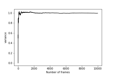
Truncation the Taylor series of the free energy at second order as we have done in this section is equivalent to assuming that a Harmonic Oscillator can be used to describe the fluctuations along our CV. The partition function, ensemble average and distribution for such systems can be calculated exactly, and there is no need for simulation. Even when the system is not harmonic, calculating the quantity we have called \(\sigma^2\) in this section is still useful as this quantity is an estimator for the variance of the distribution. For anharmonic systems, there is not a simple closed-form expression between the variance ( \(\sigma^2\)) and the second derivative of the free energy at \(\mu\) though.
The following PLUMED input splits the CV values into blocks and calculates an average from each block of data separately. We can thus use it to get information on the distribution that is being sampled when we calculate an average from sets of 500 random variables using the ideas discussed in Exercise 1: Calculating the average value of a CV.
data: READ FILEcompulsory keyword the name of the file from which to read these quantities =__FILL__ VALUEScompulsory keyword the values to read from the file =__FILL__ av: AVERAGE ARGthe input for this action is the scalar output from one or more other actions. =__FILL__ STRIDEcompulsory keyword ( default=1 ) the frequency with which the data should be collected and added to the quantity being averaged =1 CLEARcompulsory keyword ( default=0 ) the frequency with which to clear all the accumulated data. =500 PRINT ARGthe input for this action is the scalar output from one or more other actions. =__FILL__ STRIDEcompulsory keyword ( default=1 ) the frequency with which the quantities of interest should be output =__FILL__ FILEthe name of the file on which to output these quantities =colvar
Copy this input to a file called plumed.dat, fill in the blanks and run the calculation by executing the following command:
> plumed driver --noatoms
Plot a graph showing the original data from uncorrelated_data and the averages in the colvar file. You should be able to see something similar to this graph.
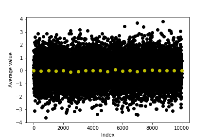
Notice how the distribution for both the black (original data) and yellow points (averages) in this graph are centred on the same quantity. Both of these quantities are thus accurate estimators for the expectation of the distribution. However, the block average that is shown in yellow is a more precise estimator for this quantity.
The reason the block average is a more precise estimator is connected to a well known result in statistics. If we compute a mean as follows:
\[ \overline{X} = \frac{1}{N} \sum_{i=1}^N X_i \]
where the \(X_i\) are all independent and identical random variables it is straghtforward to show that the expectation and variance of this random quantity are given by:
\[ \mathbb{E}(\overline{X}) = \mathbb{E}(X) \qquad \textrm{and} \qquad \textrm{var}(\overline{X}) = \frac{\textrm{var}(X)}{N} \]
where \(\mathbb{E}(X)\) and \(\textrm{var}(X)\) are the expectation and variance of the random variable \(X_i\) from which the mean was computed.
We can use the block averaging method introduced in Exercise 4: Calculating block averages to calculate error bars on the estimates of free energy. To generate 10 histograms from the data in uncorrelated_data with 100 bins starting at -4 and finishing at +4 using PLUMED we can use the input file:
data: READ FILEcompulsory keyword the name of the file from which to read these quantities =__FILL__ VALUEScompulsory keyword the values to read from the file =__FILL__ hhh: HISTOGRAM ARGthe input for this action is the scalar output from one or more other actions. =__FILL__STRIDE=1 __FILL__ could not find this keyword =-4.5 __FILL__ could not find this keyword =4.5 __FILL__ could not find this keyword =100 CLEARcompulsory keyword ( default=0 ) the frequency with which to clear all the accumulated data. =__FILL__ _FILL__ could not find this keyword =DISCRETE DUMPGRID GRIDcompulsory keyword the action that creates the grid you would like to output =__FILL__ FILEcompulsory keyword ( default=density ) the file on which to write the grid. =hist.dat STRIDEcompulsory keyword ( default=0 ) the frequency with which the grid should be output to the file. =1000
Copy this input to a file called plumed.dat, fill in the blanks and run the calculation by executing the following command:
> plumed driver --noatoms
Running this command should generate several files containing histograms that will be called: analysis.0.hist.dat, analysis.1.hist.dat etc. These files contain the histograms constructed from each of the blocks of data in your trajectory. You can merge them all to get the final free energy surface, which can be calculated using the well-known relation between the histogram, \(P(s)\), and the free energy surface, \(F(s)\), by using the following python script:
Copy this script to a cell in a python notebook and then run it on your data.
You may need to adjust the names of the files that are being read to suit your machine's setup. The graph shown in the figure below shows the free energy surface generated from the python script.
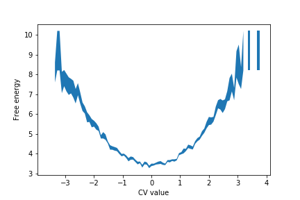
The value of the free energy in the \(i\)th bin is calculated using:
\[ F_i = -k_B T \ln \left( \frac{1}{N} \sum_{j=1}^N H_i^{(j)} \right) \]
The sum here runs over the \(N\) histograms and \(H_i^{(j)}\) is the value of \(i\)th bin in the \(j\)th estimate of the histogram. The above expression is thus calculating the logarithm of the histogram's average value in bin \(i\).
The error on the free energy, which is illustrated using the shaded region in the figure above, is calculated using:
\[ \sigma_{F_i} = \frac{k_B T}{\frac{1}{N} \sum_{j=1}^N H_i^{(j)}} \sqrt{\frac{1}{N-1} \left[ \frac{1}{N}\sum_{j=1}^N (H_i^{(j)})^2 - \left( \frac{1}{N}\sum_{j=1}^N H_i^{(j)} \right)^2 \right] } \]
The term in the square root here is the error on the average value of the histogram in bin \(i\). The error on this average can be calculated using the formulas in Exercise 4: Calculating block averages. To get the error on the free energy, we then have to propagate the errors through the expression:
\[ F(s) = - k_B T \ln\left( P(s) \right) \]
to get the expression above.
Lastly, notice that it is often useful to average the error over the grid using:
\[ \sigma = \frac{1}{M} \sum_{i=1}^M F_i \]
where the sum runs over the \(M\) bins in the histogram.
Exercise 4: Calculating block averages demonstrated one way of sampling the mean's distribution (see Exercise 1: Calculating the average value of a CV). We assumed that the \(M\) estimates of the mean were all normal random variables in the previous section but we did not need to do that. We could instead have used a non-parametric method. When using such methods we have to generate more data, which we can either do by running longer simulations, which is expensive, or by bootstrapping, which is cheaper.
We can demonstrate how bootstrapping works in practice by using the following script, which works with the first 500 points in uncorrelated_data. As you can see, we first calculate the average from all the data points. We then take new means by repeatedly sampling sets of 500 points with replacement from the data and calculating new means.
When you run the script above, it generates a file called bootstraps containing the averages that have been calculated by bootstrapping.
If you now calculate the variance from all your bootstrapped averages you should see that it close to the value you got from the expression below which was introduced in Exercise 4: Calculating block averages:
\[ \textrm{var}(\overline{X}) = \frac{\textrm{var}(X)}{N} \]
To use this expression you can insert the value of \(\textrm{var}(X)\) you computed in Exercise 3: Calculating the fluctuations for a CV with \(N=500\).
You can also use bootstrapping to estimate the errors in the free energy surface. As an additional exercise, you can try to do this form of analysis on the data in uncorrelated_data You should get a result that is similar to the result you got in Exercise 5: Free energy from block averages
In this exercise, you will review everything you have done in the previous two sections. You should:
correlated_data. Calculate the error on the average of the block average. correlated_data. Calculate the error from the bootstrap averages.You will see that the variance you obtain from the bootstrap averages is less than the variance you get by block averaging.
These variances are different because there are correlations between the data points in correlated_data. Such correlations were not present in the data set you have examined in all the exercises that appeared previously to this one. The reason this matters is that the expression:
\[ \textrm{var}(\overline{X}) = \frac{\textrm{var}(X)}{N} \]
is only valid if the random variables that \(\overline{X}\) is computed from are both identical and independent. This expression is thus not valid for correlated data. To be clear, however, we can still write:
\[ \mathbb{E}(\overline{X}) = \mathbb{E}(X) \]
as this expression holds as long as the random variables from which \(\overline{X}\) are identical. When we use this expression, the random variables only need to be independent and can be correlated.
Any data we get by computing CVs from a molecular dynamics trajectory is almost certain to contain correlations. It is thus essential to know how to handle correlated data. The block averaging technique that was introduced in Exercise 4: Calculating block averages resolves this problem. You can show that if the blocks are long enough, the averages you obtain are uncorrelated.
For the remainder of this exercise, you should use the data in correlated_data and what you have learned in the previous exercises to calculate block averages for different block sizes.
For each block size
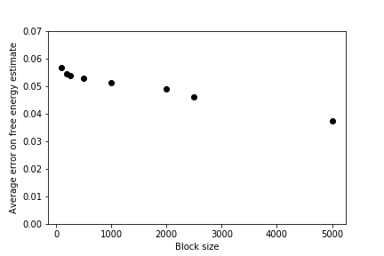
You should be able to use your data to draw a graph showing the value of the average and the associated error barm \(\epsilon\), as a function of the size of the blocks similar to the one shown below:
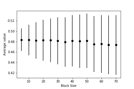
This graph shows that, when the data is correlated, the error bar is underestimated if each block average is computed from a small number of data points. When sufficient data points are used to calculate each block average, however, the error bar settles on a constant value that is independent of the block size. When this has happened you can be confident that your block averages are no longer correlated and the expression \(\textrm{var}(\overline{X}) = \frac{\textrm{var}(X)}{N}\) is thus valid.
Notice that you can also calculate the error bar using bootstrapping by selecting samples from your block averages. If you have time, you should try this. You should try to confirm that this method gives similar estimates for the error.
PLUMED is routinely used to run simulations using methods such as umbrella sampling and metadynamics. In these methods, a bias potential, \(V(x)\), is added to the Hamiltonian to enhance the sampling of phase space. CVs calculated from the frames of such biased MD simulations thus samples from the following distribution:
\[ P(s') = \frac{ \int \textrm{d}x \textrm{d}p \delta( s(x) - s') e^{-\frac{H(x,p)}{k_B T}} e^{-\frac{V(x)}{k_B T}} }{ \int \textrm{d}x\textrm{d}p e^{-\frac{H(x,p)}{k_B T}}e^{-\frac{V(x)}{k_B T}} } \]
To get information on the unbiased distribution:
\[ P(s') = \frac{ \int \textrm{d}x \textrm{d}p \delta( s(x) - s') e^{-\frac{H(x,p)}{k_B T}} }{ \int \textrm{d}x\textrm{d}p e^{-\frac{H(x,p)}{k_B T}} } \]
from such simulations we thus have to calculate weighted averages using:
\[ \overline{X}_w = \frac{\sum_{i=1}^N w_i X_i }{\sum_{i=1}^N w_i} \]
where the \(w_i\) are (random) weights that counteract the effect of the bias. The way the weights are calculated is described in PLUMED Masterclass 21.3: Umbrella sampling)
In this exercise we are going to reweight the data in weighted_data, which consists of samples from the following distribution:
\[ P(x) = \frac{1}{\sqrt{2\pi}\sigma} \exp\left( -\frac{(x-\mu)^2}{2\sigma^2} \right) \]
with \(\mu=0.6\) and \(\sigma=0.5\) with and additional constrant that \(0<x<1\). Given this information the following weighted average:
\[ \overline{X}_w = \frac{\sum_{i=1}^N w_i X_i }{\sum_{i=1}^N w_i} \qquad \textrm{where} \qquad w_i = \frac{1}{P(X_i)} \]
should be an estimator for the expectation of a uniform random variable between 0 and 1. Furthermore, the expression below:
\[ \sigma^2_{X} = \frac{V_1}{V_1-1} \sum_{i=1}^N \frac{w_i}{V_1} (x_i - \overline{X}_w)^2 \qquad \textrm{where} \qquad V_1 = \sum_{i=1}^N w_i \]
gives an estimate for the variance of the distribution after reweighting (i.e. the variance of the uniform random variable).
Notice, finally, that the tools of statistics gives us expressions for the expectation and variance of the weighted average:
\[ \mathbb{E}(\overline{X}_w) = \overline{X} \qquad \textrm{and} \qquad \textrm{var}(\overline{X}_w) = \frac{\sum_{i=1}^N w_i^2 (X_i - \overline{X}_w)^2 }{(\sum_{i=1}^N w_i)^2} \]
These expressions hold if all the \(X_i\) from which the weighted average is computed are independent and identically distributed random variables. Notice, furthermore, how the expression above for the the variance of the weighted average is not a function of the variance for the variable as was the case for the unweighted averages in Exercise 4: Calculating block averages.
In what follows we are thus going to try to extract the average and the fluctuations for the CV in the unbiased (in this case uniform) distribution as well as the unbiased free energy. We will calculate these quantities by computing weighted averages and weighted histograms from our simulation data. For the histogram we are also going to extract error bars by reweighting. To calculate these quantities using PLUMED we will use an input like this:
UNITS NATURAL( default=off ) use natural units # This ensures that Boltzmann's constant is one data: READ FILEcompulsory keyword the name of the file from which to read these quantities =__FILL__ VALUEScompulsory keyword the values to read from the file =__FILL__ # This restraint and the REWEIGHT_BIAS command after computes the weights in the formulas above. mm: RESTRAINT ARGthe input for this action is the scalar output from one or more other actions. =data ATcompulsory keyword the position of the restraint =0.6 KAPPAcompulsory keyword ( default=0.0 ) specifies that the restraint is harmonic and what the values of the force constants on each of the variables are =4 rw: REWEIGHT_BIAS TEMPthe system temperature. =1 wav: AVERAGE ARGthe input for this action is the scalar output from one or more other actions. =__FILL__ STRIDEcompulsory keyword ( default=1 ) the frequency with which the data should be collected and added to the quantity being averaged =1 LOGWEIGHTSlist of actions that calculates log weights that should be used to weight configurations when calculating averages =__FILL__ # These lines compute the variance of the random variable dd: CUSTOM ARGthe input for this action is the scalar output from one or more other actions. =data,wav FUNCcompulsory keyword the function you wish to evaluate =(x-y)*(x-y) PERIODICcompulsory keyword if the output of your function is periodic then you should specify the periodicity of the function. =NO uvar: AVERAGE ARGthe input for this action is the scalar output from one or more other actions. =dd STRIDEcompulsory keyword ( default=1 ) the frequency with which the data should be collected and added to the quantity being averaged =1 LOGWEIGHTSlist of actions that calculates log weights that should be used to weight configurations when calculating averages =rw NORMALIZATIONcompulsory keyword ( default=true ) This controls how the data is normalized it can be set equal to true, false or ndata. =false one: CONSTANT VALUEThe value of the constant =1 wsum: AVERAGE ARGthe input for this action is the scalar output from one or more other actions. =one STRIDEcompulsory keyword ( default=1 ) the frequency with which the data should be collected and added to the quantity being averaged =1 LOGWEIGHTSlist of actions that calculates log weights that should be used to weight configurations when calculating averages =rw NORMALIZATIONcompulsory keyword ( default=true ) This controls how the data is normalized it can be set equal to true, false or ndata. =false var: CUSTOM ARGthe input for this action is the scalar output from one or more other actions. =uvar,wsum FUNCcompulsory keyword the function you wish to evaluate =x/(y-1) PERIODICcompulsory keyword if the output of your function is periodic then you should specify the periodicity of the function. =NO # Print out the average and variance of the uniform random variable PRINT ARGthe input for this action is the scalar output from one or more other actions. =__FILL__ STRIDEcompulsory keyword ( default=1 ) the frequency with which the quantities of interest should be output =1 FILEthe name of the file on which to output these quantities =colvar # Construct the histogram hhh: HISTOGRAM ARGthe input for this action is the scalar output from one or more other actions. =__FILL__ LOGWEIGHTSlist of actions that calculates log weights that should be used to weight configurations when calculating averages =__FILL__ __FILL__ could not find this keyword =0 __FILL__ could not find this keyword =1 __FILL__ could not find this keyword =20 CLEARcompulsory keyword ( default=0 ) the frequency with which to clear all the accumulated data. =__FILL__ NORMALIZATIONcompulsory keyword ( default=ndata ) This controls how the data is normalized it can be set equal to true, false or ndata. =true __FILL__ could not find this keyword =DISCRETE DUMPGRID GRIDcompulsory keyword the action that creates the grid you would like to output =__FILL__ FILEcompulsory keyword ( default=density ) the file on which to write the grid. =hist.dat STRIDEcompulsory keyword ( default=0 ) the frequency with which the grid should be output to the file. =1000
Copy this input to a file called plumed.dat, fill in the blanks and run the calculation by executing the following command:
> plumed driver --noatoms
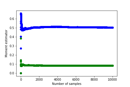
I obtained the following graphs showing how the mean and variance change with sample size.
The free energy with errors from this data looks like this:
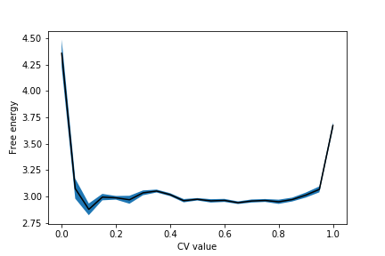
It is up to you to work out how to adapt the script given in Exercise 5: Free energy from block averages, so it works here. The script above works for unweighted means. Here, however, you have to calculate weighted means using the formulas above.
We can now bring all this together by running a metadynamics simulation and extracting the free energy surface by reweighting. The other exercises in this tutorial have shown us that when we do this, it is essential to:
As these three issues have been the focus of this tutorial, we focus on them in the exercise that follows. The theory behind the metadynamics method that we are using is discussed in detail in PLUMED Masterclass 21.4: Metadynamics if you are interested.
We will study a system of 7 Lennard Jones atoms in two dimensions in what follows using the MD code simplemd that is part of PLUMED. You can run this code by issuing the command:
plumed simplemd < in
where in here is the input file from the GitHub repository for this tutorial. This input file instructs PLUMED to perform 200000 steps of MD at a temperature of \(k_B T = 0.1 \epsilon\) starting from the configuration in input.xyz.
The timestep in this simulation is 0.005 \(\sqrt{\epsilon}{m\sigma^2}\) and the temperature is kept fixed using a Langevin thermostat with a relaxation time of \(0.1 \sqrt{\epsilon}{m\sigma^2}\). Trajectory frames are output every 1000 MD steps to a file called trajectory.xyz. Notice also that to run the calculation above you need to provide a PLUMED input file called plumed.dat.
We want to investigate transitions between the four structures of Lennard Jones 7 that are shown below using metadynamics.

However, when we run the metadynamics, we will often find that the cluster evaporates and the seven atoms separate. To prevent this, we will thus add restraints to prevent the cluster from evaporating. The particular restraint we are going to use will prevent all the atoms from moving more than \(2\sigma\) from the centre of mass of the cluster. As the masses of all the atoms in the cluster are the same, we can compute the position of the centre of mass using:
\[ \mathbf{x}_\textrm{com} = \frac{1}{N} \sum_{i=1}^N \mathbf{x}_i \]
where \(\mathbf{x}_i\) is the position of the atom with the index \(i\). The distance between the atom with index \(i\) and the position of this centre of mass, \(d_i\), can be computed using Pythagoras' theorem. These distances are then restrained by using the following potential:
\[ V(d_i) = \begin{cases} 100*(d_i-2.0)^2 & \textrm{if} \quad d_i > 2 \\ 0 & \textrm{otherwise} \end{cases} \]
as you can see, this potential does not affect the dynamics when these distances are less than 2 \(\epsilon\). If an atom is more than 2 \(\epsilon\) from the centre of mass, however, this potential will drive it back towards the centre of mass.
A metadynamics bias will be used to force the system to move between the four configurations shown in masterclass-21-1-4-lj7-minima. This bias will act on the second and third central moments of the distribution of coordination numbers. The nth central moment of a set of numbers, \(\{X_i\}\) can be calculated using:
\[ \mu^n = \frac{1}{N} \sum_{i=1}^N ( X_i - \langle X \rangle )^n \qquad \textrm{where} \qquad \langle X \rangle = \frac{1}{N} \sum_{i=1}^N X_i \]
Furthermore, we can compute the coordination number of our Lennard Jones atoms using:
\[ c_i = \sum_{i \ne j } \frac{1 - \left(\frac{r_{ij}}{1.5}\right)^8}{1 - \left(\frac{r_{ij}}{1.5}\right)^{16} } \]
where \(r_{ij}\) is the distance between atom \(i\) and atom \(j\). With all this information in mind the following cell contains a skeleton input file for PLUMED that gets it to perform metadynamics using the second and third central moments of the distribution of coordination numbers as a CV.
# this optional command tells VIM that this is a PLUMED file and to colour the text accordingly # vim: ft=plumed # This tells PLUMED we are using Lennard Jones units UNITS NATURAL( default=off ) use natural units # Calculate the position of the centre of mass. We can then refer to this position later in the input using the label com. com: COM __FILL__ # Add the restraint on the distance between com and the first atom d1: DISTANCE __FILL__ UPPER_WALLS ARGthe input for this action is the scalar output from one or more other actions. =d1 __FILL__ # Add the restraint on the distance between com and the second atom d2: DISTANCE __FILL__ UPPER_WALLS __FILL__ # Add the restraint on the distance between com and the third atom d3: DISTANCE __FILL__ UPPER_WALLS __FILL__ # Add the restraint on the distance between com and the fourth atom d4: DISTANCE __FILL__ UPPER_WALLS __FILL__ # Add the restraint on the distance between com and the fifth atom d5: DISTANCE __FILL__ UPPER_WALLS __FILL__ # Add the restraint on the distance between com and the sixth atom d6: DISTANCE __FILL__ UPPER_WALLS __FILL__ # Add the restraint on the distance between com and the seventh atom d7: DISTANCE __FILL__ UPPER_WALLS __FILL__ # Calculate the collective variables c1: COORDINATIONNUMBER SPECIESthis keyword is used for colvars such as coordination number. =__FILL__ MOMENTScalculate the moments of the distribution of collective variables. =__FILL__ SWITCHThis keyword is used if you want to employ an alternative to the continuous switching function defined above. ={RATIONAL __FILL__ } # Do metadynamics METAD ARGthe input for this action is the scalar output from one or more other actions. =__FILL__ HEIGHTthe heights of the Gaussian hills. =__FILL__ PACEcompulsory keyword the frequency for hill addition =__FILL__ SIGMAcompulsory keyword the widths of the Gaussian hills =__FILL__ GRID_MINthe lower bounds for the grid =-1.5,-1.5 GRID_MAXthe upper bounds for the grid =2.5,2.5 GRID_BINthe number of bins for the grid =500,500 BIASFACTORuse well tempered metadynamics and use this bias factor. =5
Copy this input to file called plumed.dat and modify it so that it instructs PLUMED to add Gaussian kernels with a bandwidth of 0.1 in both the second and third moment of the distribution of coordination numbers and a height of 0.05 \(\epsilon\) every 500 MD steps. You can then use this input together with the input.xyz, and in files, you obtained from the GitHub repository to generate a metadynamics trajectory at \(k_B T = 0.1 \epsilon\) by running the command:
plumed simplemd < in
Once you have run the metadynamics calculations, you can post-process the output trajectory using driver to extract the free energy by reweighting. Notice that to do block averaging, you will need to extract multiple estimates for the (weighted) histogram. You should thus use the following input file to extract estimates of the histogram:
# this optional command tells VIM that this is a PLUMED file and to colour the text accordingly # vim: ft=plumed UNITS NATURAL( default=off ) use natural units # We can delete the parts of the input that specified the walls and disregard these in our analysis # It is OK to do this as we are only interested in the value of the free energy in parts of phase space # where the bias due to these walls is not acting. c1: COORDINATIONNUMBER SPECIESthis keyword is used for colvars such as coordination number. =__FILL__ MOMENTScalculate the moments of the distribution of collective variables. =__FILL__ SWITCHThis keyword is used if you want to employ an alternative to the continuous switching function defined above. ={RATIONAL __FILL__} # The metadynamics bias is restarted here so we consider the final bias as a static bias in our calculations METAD ARGthe input for this action is the scalar output from one or more other actions. =__FILL__ HEIGHTthe heights of the Gaussian hills. =0.05 PACEcompulsory keyword the frequency for hill addition =50000000 SIGMAcompulsory keyword the widths of the Gaussian hills =0.1,0.1 GRID_MINthe lower bounds for the grid =-1.5,-1.5 GRID_MAXthe upper bounds for the grid =2.5,2.5 GRID_BINthe number of bins for the grid =500,500 TEMPthe system temperature - this is only needed if you are doing well-tempered metadynamics =0.1 BIASFACTORuse well tempered metadynamics and use this bias factor. =5 RESTARTallows per-action setting of restart (YES/NO/AUTO) =YES # This adjusts the weights of the sampled configurations and thereby accounts for the effect of the bias potential rw: REWEIGHT_BIAS TEMPthe system temperature. =0.1 # Calculate the histogram and output it to a file hh: HISTOGRAM ARGthe input for this action is the scalar output from one or more other actions. =c1.* GRID_MINcompulsory keyword the lower bounds for the grid =-1.5,-1.5 GRID_MAXcompulsory keyword the upper bounds for the grid =2.5,2.5 GRID_BINthe number of bins for the grid =200,200 BANDWIDTHcompulsory keyword the bandwidths for kernel density estimation =0.02,0.02 LOGWEIGHTSlist of actions that calculates log weights that should be used to weight configurations when calculating averages =__FILL__ CLEARcompulsory keyword ( default=0 ) the frequency with which to clear all the accumulated data. =__FILL__ NORMALIZATIONcompulsory keyword ( default=ndata ) This controls how the data is normalized it can be set equal to true, false or ndata. =true DUMPGRID GRIDcompulsory keyword the action that creates the grid you would like to output =hh FILEcompulsory keyword ( default=density ) the file on which to write the grid. =my_histogram.dat STRIDEcompulsory keyword ( default=0 ) the frequency with which the grid should be output to the file. =2500
Once you have filled in the blanks in this input, you can then run the calculation by using the command:
> plumed driver --ixyz trajectory.xyz --initial-step 1
You must make sure that the HILLS file that was output by your metadynamics simulation is available in the directory where you run the above command.
For the rest of the exercise, you are on your own. You must use what you have learned in the other parts of the tutorial to generate plots similar to those shown below. The leftmost plot here is the free energy surface computed by taking the (weighted) average of the blocks, the right panel shows the size of the error bar on the free energy at each point of the free energy surface.
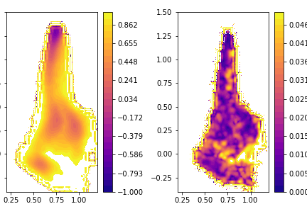
Notice that the data is correlated here so you should investigate how the error size depends on the lengths of the blocks as was discussed in Exercise 7: Dealing with correlated data. When I did this analysis I found that the error does not have a strong dependence on the size of the blocks.
Finally, if you are struggling to plot the 2D free energy surface, you can generate free energy as a function of one CV only using the ideas from earlier exercises.
Hint: You are now calculating weighted averages so you will need to use the code you wrote for Exercise 8: Weighted averages to merge the histograms
If you want to know more about good practise using PLUMED you can read https://arxiv.org/abs/1812.08213. We would also recommend learning about kernel density estimation, which will often give you smoother histograms. You can start learning about kernel density estimation by reading https://en.wikipedia.org/wiki/Kernel_density_estimation. My full sets of notes are available here:
 1.8.17